|
Special Issue:
SPECIAL TOPIC — Machine learning in statistical physics
|
|
|
|
Restricted Boltzmann machine: Recent advances and mean-field theory |
Aurélien Decelle1,2,?( ), Cyril Furtlehner2 ), Cyril Furtlehner2 |
1Departamento de Física Téorica I, Universidad Complutense, 28040 Madrid, Spain
1TAU team INRIA Saclay & LISN Université Paris Saclay, Orsay 91405, France |
|
|
|
|
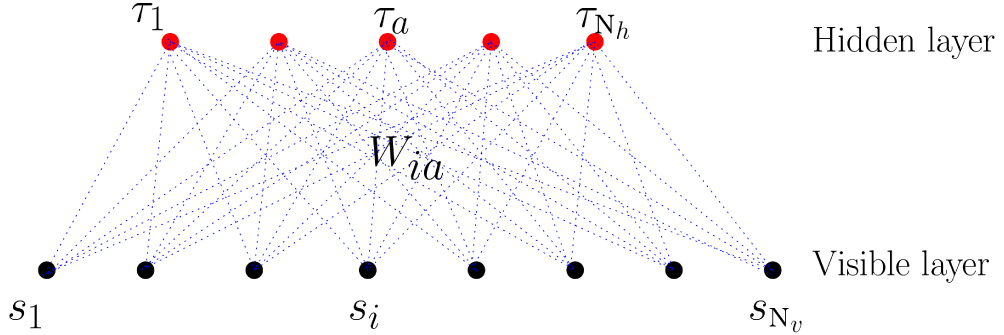
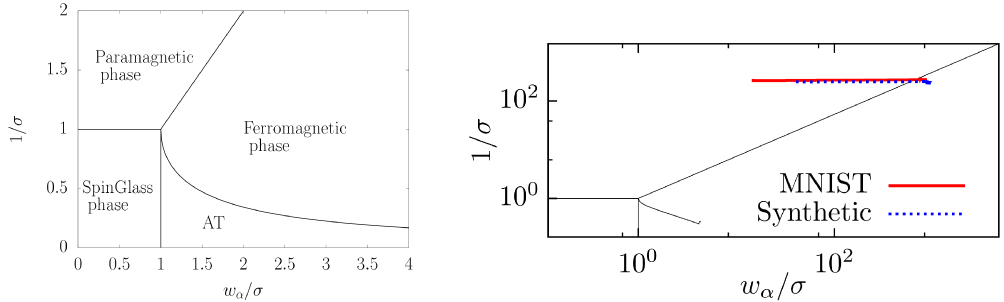
Abstract This review deals with restricted Boltzmann machine (RBM) under the light of statistical physics. The RBM is a classical family of machine learning (ML) models which played a central role in the development of deep learning. Viewing it as a spin glass model and exhibiting various links with other models of statistical physics, we gather recent results dealing with mean-field theory in this context. First the functioning of the RBM can be analyzed via the phase diagrams obtained for various statistical ensembles of RBM, leading in particular to identify a compositional phase where a small number of features or modes are combined to form complex patterns. Then we discuss recent works either able to devise mean-field based learning algorithms; either able to reproduce generic aspects of the learning process from some ensemble dynamics equations or/and from linear stability arguments.
|
Received: 30 September 2020
Accepted manuscript online:
|
| Fund: *AD was supported by the Comunidad de Madrid and the Complutense University of Madrid (Spain) through the Atracción de Talento program (Ref. 2019-T1/TIC-13298). |
Cite this article:
Aurélien Decelle, Cyril Furtlehner Restricted Boltzmann machine: Recent advances and mean-field theory 2021 Chin. Phys. B 30 040202
|
[1] Goodfellow I, Bengio Y, Courville A, Bengio Y 2016 Deep learning 1 Cambridge MIT Press
[2] Mehta P, Bukov M, Wang C H, Day A G R, Richardson C, Fisher C K, Schwab D J 2019 Physics Reports 810 1
[3] Ronneberger O, Fischer P, Brox T 2015 In International Conference on Medical image computing and computer-assisted intervention 234 241 Springer
[4] Carrasquilla J, Melko R G 2017 Nat. Phys. 13 431
[5] Smolensky P 1986 In Parallel Distributed Processing 1 Rumelhart D, McLelland J 194 281 MIT Press
[6] Hinton G E 2002 Neural Computation 14 1771
[7] Ackley D H, Hinton G E, Sejnowski T J 1985 Cognitive Science 9 147
[8] LeCun Y, Bottou L, Bengio Y, Haffner P 1998 Proc. IEEE 86 2278
[9] Le Roux N, Bengio Y 2008 Neural Computation 20 1631
[10] Montfar G 2016 Restricted boltzmann machines: Introduction and review. In Information Geometry and Its Applications IV 75 115 Springer
[11] Salakhutdinov R, Hinton G 2009 Deep Boltzmann machines. In Artificial intelligence and statistics 448 455
[12] Krizhevsky A, Hinton G et al. 2009 Learning multiple layers of features from tiny images. Technical report Citeseer
[13] Yasuda M, Tanaka K 2009 Neural Computation 21 3130
[14] Cho K, Ilin A, Raiko T 2011 Improved learning of Gaussian-Bernoulli restricted Boltzmann machines. In International conference on artificial neural networks 10 17 Springer
[15] Yamashita T, Tanaka M, Yoshida E, Yamauchi Y, Fujiyoshii H 2014 To be Bernoulli or to be Gaussian, for a restricted Boltzmann machine. In 2014 22nd International Conference on Pattern Recognition 1520 1525 IEEE
[16] Hjelm R D, Calhoun V D, Salakhutdinov R, Allen E A, Adali T, Plis S M 2014 NeuroImage 96 245
[17] Hu X, Huang H, Peng B, Han J, Liu N, Lv J, Guo L, Guo C, Liu T 2018 Human brain mapping 39 2368
[18] Goodfellow I, Pouget-Abadie J, Mirza M, Xu B, Warde-Farley D, Ozair S, Courville A, Bengio Y 2014 Generative adversarial nets. In Advances in neural information processing systems 2672 2680
[19] Yelmen B, Decelle A, Ongaro L, Marnetto D, Tallec C, Montinaro F, Furtlehner C, Pagani L, Jay F 2021 PLoS genetics 17 e1009303
[20] Zhang N, Ding S F, Zhang J, Xue Y 2018 Neurocomputing 275 1186
[21] Cho KyungHyun, Raiko T, Ilin A 2011 Enhanced gradient and adaptive learning rate for training restricted Boltzmann machines In ICML
[22] Tang Y C, Sutskever I 2011 Data normalization in the learning of restricted Boltzmann machines Department of Computer Science University of Toronto Technical Report UTML-TR-11-2
[23] Hopfield J J 1982 Proc. Natl. Acad. Sci. 79 2554
[24] Amit D J, Gutfreund H, Sompolinsky H 1985 Phys. Rev. A 32 1007
[25] Amit D J, Gutfreund H, Sompolinsky H 1985 Phys. Rev. Lett. 55 1530
[26] Amit D J, Gutfreund H, Sompolinsky H 1987 Annals of Physics 173 30
[27] Rosenblatt F 1958 Psychological Review 65 386
[28] Gardner E 1988 J. Phys. A: Math. Gen. 21 257
[29] Gardner E, Derrida B 1988 J. Phys. A: Math. Gen. 21 271
[30] Mzard M, Parisi G, Virasoro M 1987 Spin glass theory and beyond: An Introduction to the Replica Method and Its Applications 9 World Scientific Publishing Company
[31] Carreira-Perpinan M A, Hinton G E 2005 On contrastive divergence learning In Aistats 10 33 40 Citeseer
[32] Tieleman T 2008 Training restricted Boltzmann machines using approximations to the likelihood gradient. In Proceedings of the 25th international conference on Machine learning 1064 1071
[33] Fischer A, Igel C 2014 Pattern Recognition 47 25
[34] Karakida R, Okada M, Amari S I 2014 Analyzing feature extraction by contrastive divergence learning in rbms. In Deep learning and representation learning workshop: NIPS
[35] Karakida R, Okada M, Amari S I 2016 Neural Networks 79 78
[36] Decelle A, Fissore G, Furtlehner C 2018 J. Stat. Phys. 172 1576
[37] Decelle A, Fissore G, Furtlehner C 2017 Europhys. Lett. 119 60001
[38] Berlin T H, Kac M 1952 Phys. Rev. 86 821
[39] Stanley H E 1968 Phys. Rev. 176 718
[40] Decelle A, Furtlehner C 2020 J. Phys. A: Math. Theor. 53 184002
[41] Genovese G, Tantari D 2020 J. Phys. A: Math. Theor. 53 094001
[42] Nijman M J, Kappen H J 1997 International Journal of Neural Systems 8 301
[43] MacKay D J C, David J C 2003 Information theory, inference and learning algorithms Cambridge university press
[44] Bishop C M 2006 Pattern recognition and machine learning Springer
[45] Rose K, Gurewitz E, Fox G C 1990 Phys. Rev. Lett. 65 945
[46] Kloppenburg M, Tavan P 1997 Phys. Rev. E 55 2089
[47] Akaho S, Kappen H J 2000 Neural Computation 12 1411
[48] Barra A, Bernacchia A, Santucci E, Contucci P 2012 Neural Networks 34 1
[49] Mzard M 2017 Phys. Rev. E 95 022117
[50] Shimagaki K, Weigt M 2019 Phys. Rev. E 100 032128
[51] Decelle A, Hwang S, Rocchi J, Tantari D 2019 arXiv:1906.11988
[52] Hyv?rinen A, Oja E 2000 Neural Networks 13 411
[53] Yuuki Y, Tomu K, Muneki Y 2000 The Review of Socionetwork Strategies 13 253
[54] Hahnloser R H R, Sarpeshkar R, Mahowald M A, Douglas R J, Seung H S 2000 Nature 405 947
[55] Teh Y W, Hinton G E 2001 Rate-coded restricted Boltzmann machines for face recognition. In Advances in neural information processing systems 908 914
[56] Nair V, Hinton G E 2010 Rectified linear units improve restricted Boltzmann machines. In Proceedings of the 27th international conference on machine learning (ICML-10) 807 814
[57] Barra A, Genovese G, Sollich P, Tantari D 2018 Phys. Rev. E 97 022310
[58] Tubiana J, Monasson R 2017 Phys. Rev. Lett. 118 138301
[59] Huang H P 2017 J. Stat. Mech.: Theor. Exper. 2017 053302
[60] Tubiana J 2018 Restricted Boltzmann machines: from compositional representations to protein sequence analysis PhD thesis, ENS Thse de doctorat dirige par Monasson, Rmi et Cocco, Simona Physique Paris Sciences et Lettres
[61] Agliari E, Barra A, Tirozzi B 2019 J. Stat. Mech.: Theor. Exper. 2019 033301
[62] Hartnett G S, Parker E, Geist E 2018 Phys. Rev. E 98 022116
[63] Agliari E, Barra A, Galluzzi A, Guerra F, Moauro F 2012 Phys. Rev. Lett. 109 268101
[64] Agliari E, Barra A, Galluzzi A, Isopi M 2014 Neural Networks 49 19
[65] Wemmenhove B, Coolen A C C 2003 J. Phys. A: Math. Gen. 36 9617
[66] Huang H P 2018 J. Phys. A: Math. Theor. 51 08LT01
[67] Kirkpatrick S, Sherrington D 1978 Phys. Rev. B 17 4384
[68] Amari S I 1977 Biol. Cybern. 26 175
[69] Harsh M, Tubiana J, Cocco S, Monasson R 2020 J. Phys. A: Math. Theor. 53 174002
[70] Hukushima K, Nemoto K 1996 J. Phys. Soc. Jpn. 65 1604
[71] Desjardins G, Courville A, Bengio Y, Vincent P, Delalleau O 2010 Parallel tempering for training of restricted Boltzmann machines. In Proceedings of the thirteenth international conference on artificial intelligence and statistics 145 152 Cambridge MIT Press
[72] Chako T, Muneki Y 2016 J. Phys. Soc. Jpn. 85 034001
[73] Gabri M, Tramel E W, Krzakala F 2015 Training restricted Boltzmann machine via the Thouless-Anderson-Palmer free energy. In Advances in neural information processing systems 640 648
[74] Tramel E W, Gabri M, Manoel A, Caltagirone F, Krzakala F 2018 Phys. Rev. X 8 041006
[75] Thouless D J, Anderson P W, Palmer R G 1977 Philosophical Magazine 35 593
[76] Plefka T 1982 J. Phys. A: Math. Gen. 15 1971
[77] Georges A, Yedidia J S 1991 J. Phys. A: Math. Gen. 24 2173
[78] Maillard A, Foini L, Castellanos A L, Krzakala F, Mzard M, Zdeborov L 2019 J. Stat. Mech.: Theor. Exp. 2019 113301
[79] Tramel E W, Manoel A, Caltagirone F, Gabri M, Krzakala F 2016 Inferring sparsity: Compressed sensing using generalized restricted Boltzmann machines. In 2016 IEEE Information Theory Workshop (ITW) 265 269
[80] Fissore G, Decelle A, Furtlehner C, Han Y F 1912.09382 2019 arXiv:
[81] Huang H P, Toyoizumi T 2015 Phys. Rev. E 91 050101
[82] Lage-Castellanos A, Mulet R, Ricci-Tersenghi F, Rizzo T 2013 J. Phys. A: Math. Theor. 46 135001
[83] Ricci-Tersenghi F 2012 J. Stat. Mech.: Theor. Exp. 2012 P08015
[84] Nguyen H C, Berg J 2012 J. Stat. Mech.: Theor. Exp. 2012 P03004
[85] Huang H P, Toyoizumi T 2016 Phys. Rev. E 94 062310
[86] Huang H P 2020 Phys. Rev. E 102 030301
[87] Salakhutdinov R, Murray I 2008 On the quantitative analysis of deep belief networks. In Proceedings of the 25th international conference on Machine learning 872 879
[88] Krause O, Fischer A, Igel C 2020 Artificial Intelligence 278 103195
[89] Yale A, Dash S, Dutta R, Guyon I, Pavao A, Bennett K P 2020 Generation and evaluation of privacy preserving synthetic health data Neurocomputing |
| No Suggested Reading articles found! |
|
|
Viewed |
|
|
|
Full text
|
|
|
|
|
Abstract
|
|
|
|
|
Cited |
|
|
|
|
Altmetric
|
|
blogs
Facebook pages
Wikipedia page
Google+ users
|
Online attention
Altmetric calculates a score based on the online attention an article receives. Each coloured thread in the circle represents a different type of online attention. The number in the centre is the Altmetric score. Social media and mainstream news media are the main sources that calculate the score. Reference managers such as Mendeley are also tracked but do not contribute to the score. Older articles often score higher because they have had more time to get noticed. To account for this, Altmetric has included the context data for other articles of a similar age.
View more on Altmetrics
|
|
|