Lattice configurations in spin-1 Bose–Einstein condensates with the SU(3) spin–orbit coupling

doi:10.1088/1674-1056/abab72

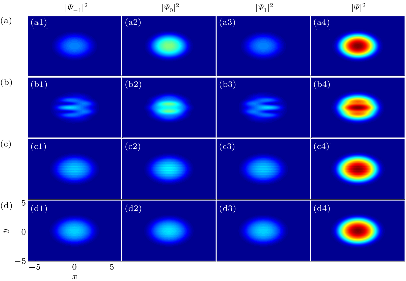
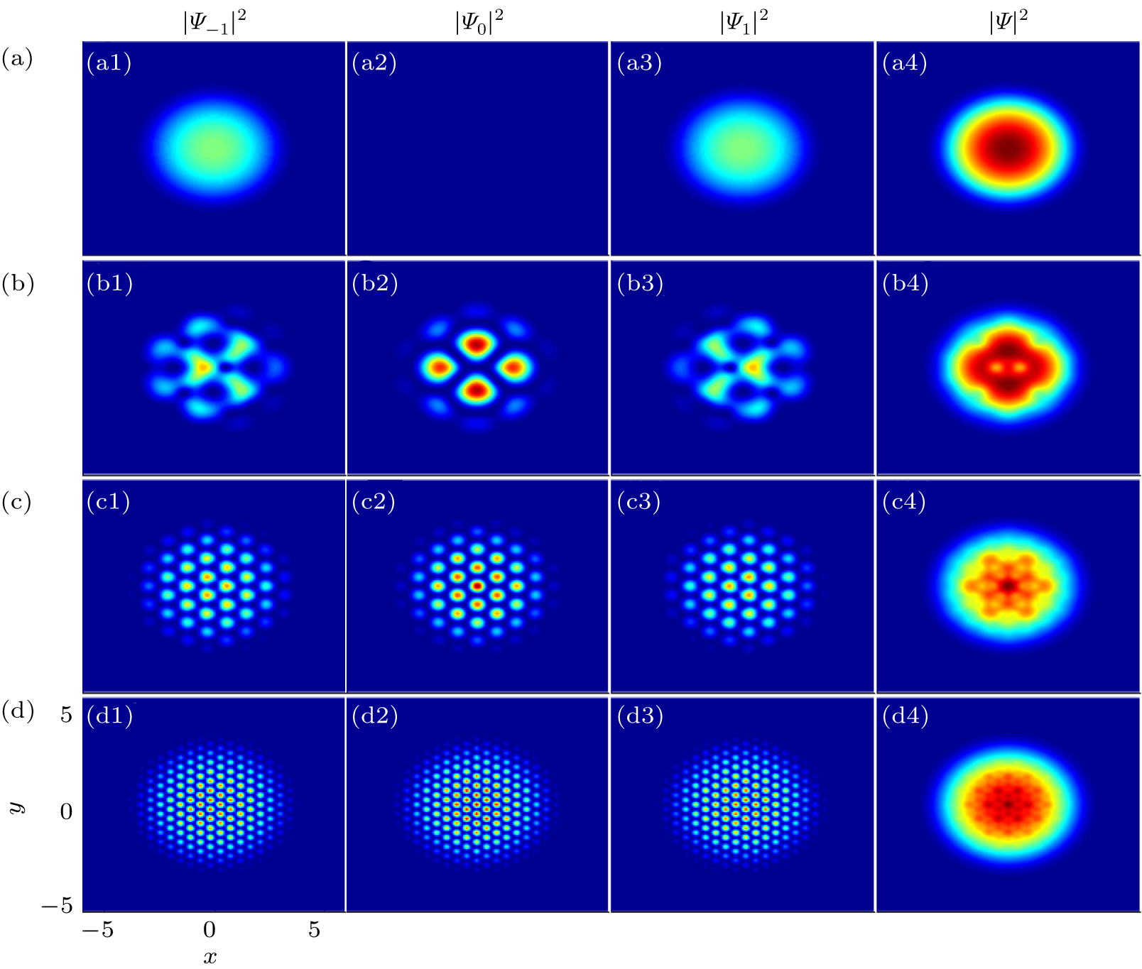
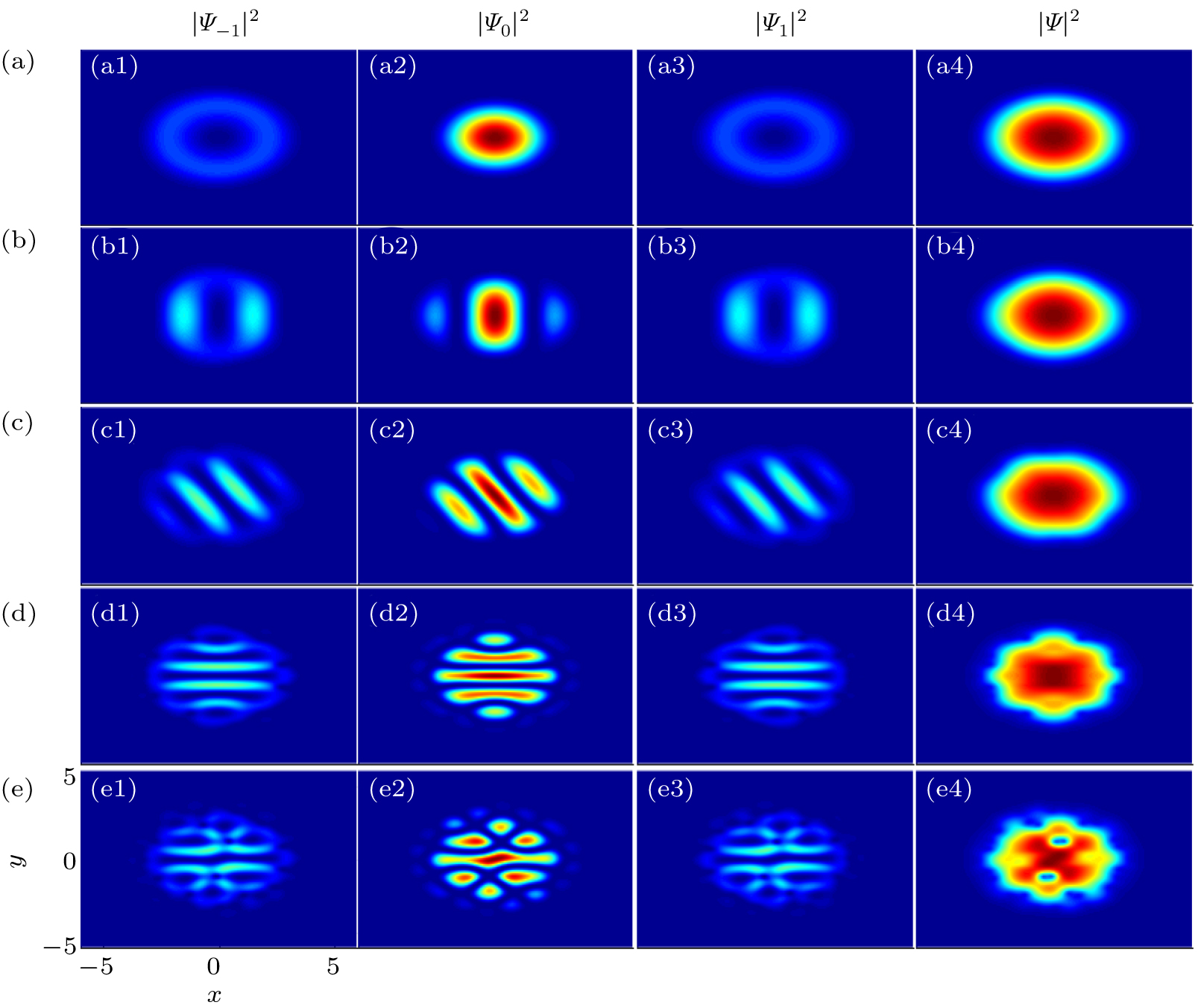
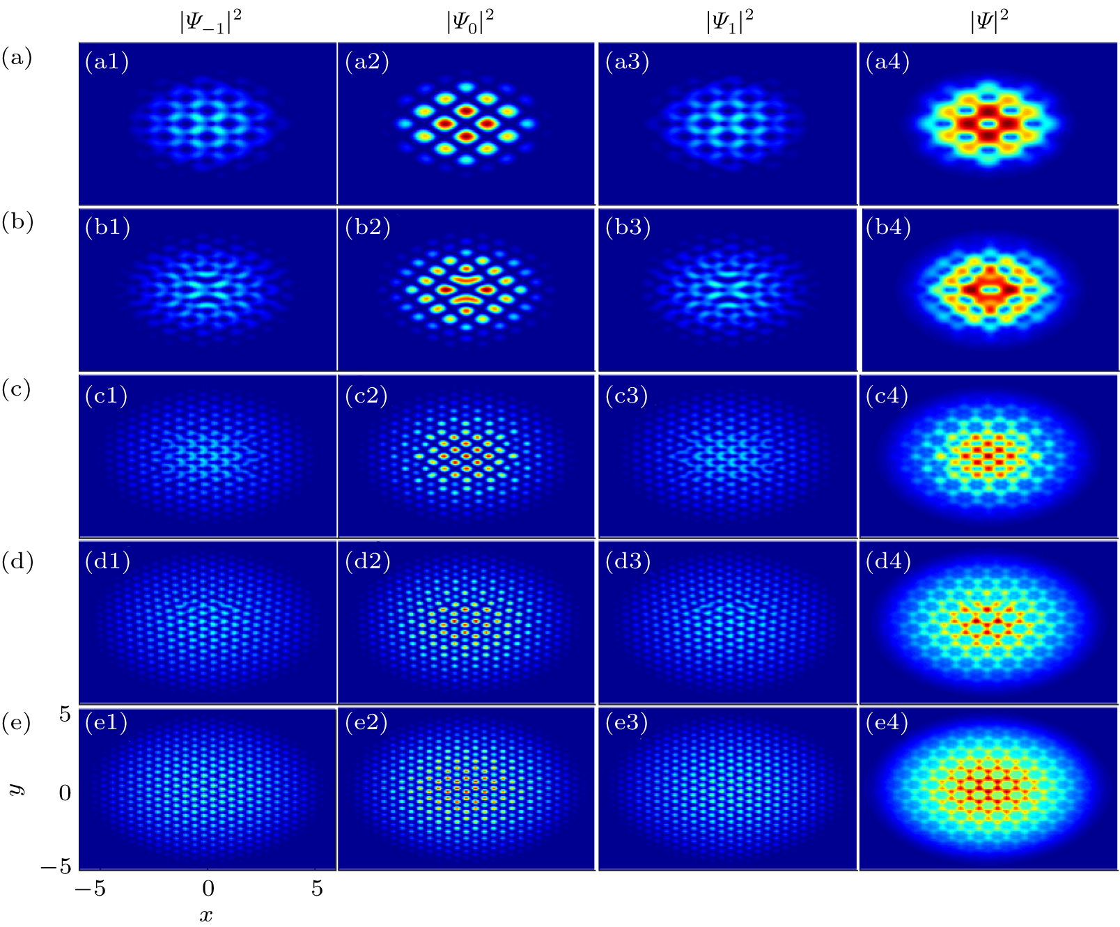
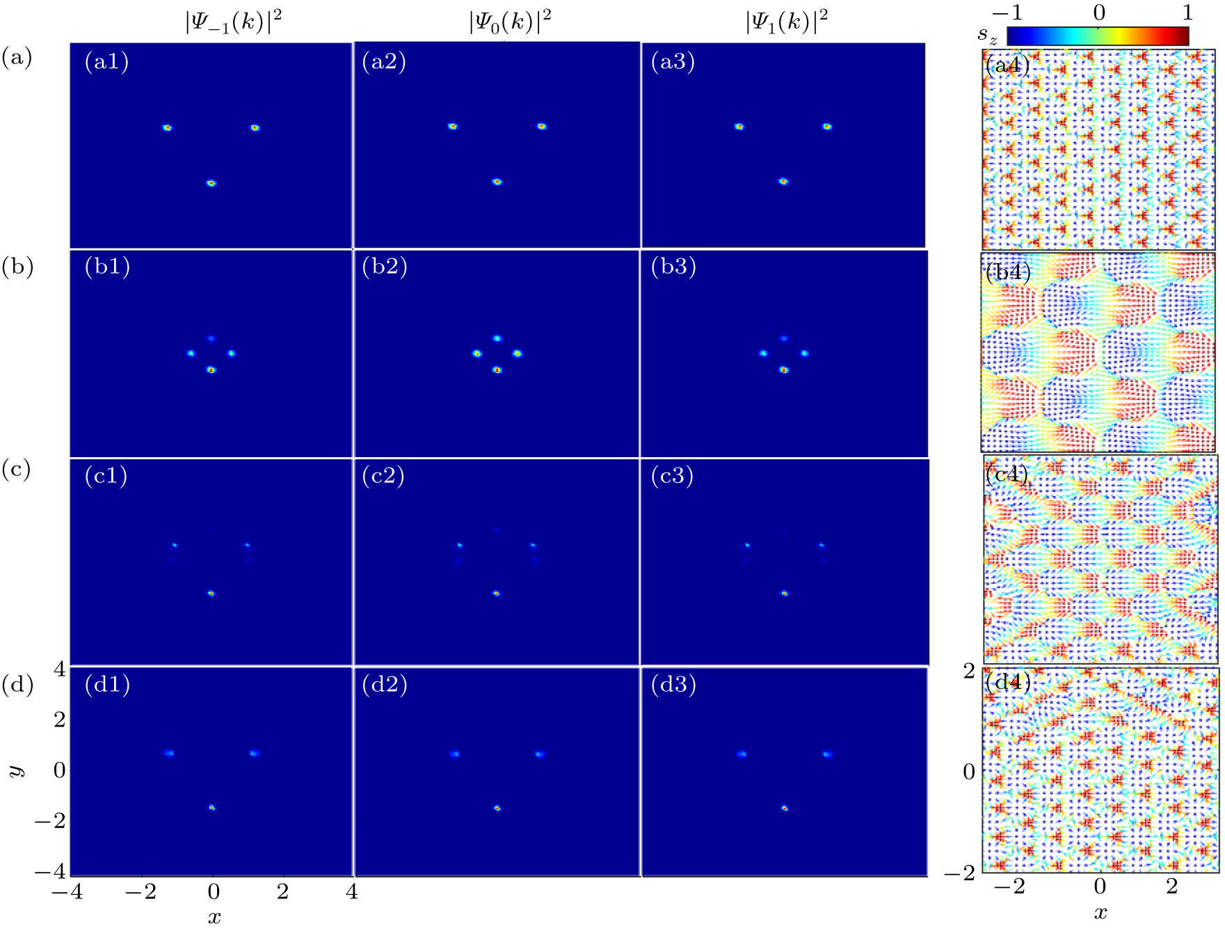
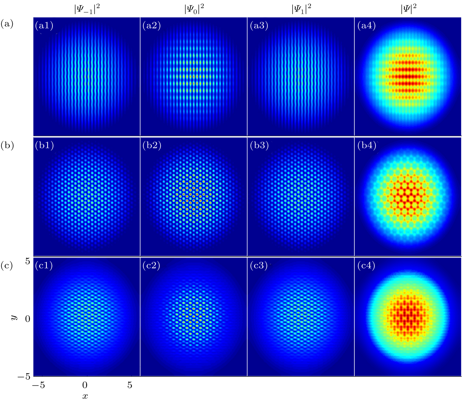
Abstract

We consider the SU(3) spin–orbit coupled spin-1 Bose–Einstein condensates in a two-dimensional harmonic trap. The competition between the SU(3) spin–orbit coupling and the spin-exchange interaction results in a rich variety of lattice configurations. The ground-state phase diagram spanned by the isotropic SU(3) spin–orbit coupling and the spin–spin interaction is presented. Five ground-state phases can be identified on the phase diagram, including the plane wave phase, the stripe phase, the kagome lattice phase, the stripe-honeycomb lattice phase, and the honeycomb hexagonal lattice phase. The system undergoes a sequence of phase transitions from the rectangular lattice phase to the honeycomb hexagonal lattice phase, and to the triangular lattice phase in spin-1 Bose–Einstein condensates with anisotrpic SU(3) spin–orbit coupling.

Keywords: Bose-Einstein condensates lattice configurations SU(3) spin-orbit coupling

Received: 06 April 2020
Revised: 02 July 2020
Accepted manuscript online: 01 August 2020

PACS:	03.75.Lm	(Tunneling, Josephson effect, Bose-Einstein condensates in periodic potentials, solitons, vortices, and topological excitations)
	03.75.Mn	(Multicomponent condensates; spinor condensates)
	67.85.Hj	(Bose-Einstein condensates in optical potentials)
	67.80.K-	(Other supersolids)

Corresponding Authors: ^†Corresponding author. E-mail: wangjiguo@stdu.edu.cn

About author:

†Corresponding author. E-mail: wangjiguo@stdu.edu.cn

* Project supported by the National Natural Science Foundation of China (Grant No. 11904242) and the Natural Science Foundation of Hebei Province, China (Grant No. A2019210280).

Cite this article:

Ji-Guo Wang(王继国)†, Yue-Qing Li(李月晴), and Yu-Fei Dong(董雨菲) Lattice configurations in spin-1 Bose–Einstein condensates with the SU(3) spin–orbit coupling 2020 Chin. Phys. B 29 100304

Fig. 1.

The ground-state density profiles of ferromagnetic spin-1 BECs with isotropic SU(3) SOC. The columns in every panel from left to right are the densities of the m_F = –1 component |Ψ₋₁|², the m_F = 0 component |Ψ₀|², the m_F = 1 component |Ψ₁|², and the total |Ψ|² = |Ψ₋₁|²+|Ψ₀|²+|Ψ₁|². The SOC strengths in (a)–(d) are γ = 0, 1, 3, and 5, respectively. The spin–spin interaction c₂ = −50.

Fig. 2.

The ground-state density profiles of antiferromagnetic spin-1 BECs with isotropic SU(3) SOC. The columns in every panel from left to right are the densities of the m_F = –1 component |Ψ₋₁|², the m_F = 0 component |Ψ₀|², the m_F = 1 component |Ψ₁|², and the total |Ψ|² = |Ψ₋₁|²+|Ψ₀|²+|Ψ₁|². The SOC strengths in (a)–(d) are γ = 0, 1, 2, and 4, respectively. The spin–spin interaction c₂ = 100.

Fig. 3.

The ground-state density profiles of antiferromagnetic spin-1 BECs with isotropic SU(3) SOC. The columns in every panel from left to right are the densities of the m_F = –1 component |Ψ₋₁|², the m_F = 0 component |Ψ₀|², the m_F = 1 component |Ψ₁|², and the total |Ψ|² = |Ψ₋₁|²+|Ψ₀|²+|Ψ₁|². The SOC strengths in (a)–(e) are γ = 0.50, 0.75, 1.10, 1.65, and 1.75, respectively. The spin–spin interaction c₂ = 2000.

Fig. 4.

The ground-state density profiles of antiferromagnetic spin-1 BECs with isotropic SU(3) SOC. The columns in every panel from left to right are the densities of m_F = –1 component |Ψ₋₁|², m_F = 0 component |Ψ₀|², m_F = 1 component |Ψ₁|², and the total |Ψ|² = |Ψ₋₁|²+|Ψ₀|²+|Ψ₁|². The SOC strengths in (a)-(e) are γ = 2, 2.5, 3.5, 4, and 4.4, respectively. The spin–spin interaction c₂ = 2000.

Fig. 5.

The parameters of (a)–(d) are the same as those of Figs. 2(d), 4(a), 4(b), and 4(e), respectively. The momentum distributions of (b1)–(d1) the m_F = –1 component |Ψ₋₁(k)|², (b2)–(d2) the m_F = 0 component |Ψ₀(k)|², and (b3)–(d3) the m_F = 1 component |Ψ₁(k)|².

Fig. 6.

The ground-state phase diagram spanned by the SU(3) SOC strength γ and the spin–spin interaction strength c₂. Five ground-state phases can be identified on the phase diagram, including the PW phase, the ST phase, the KL phase, the SHL phase, and the HHL phase.

Fig. 7.

The ground-state density profiles of spin-1 antiferromagnetic BECs with anisotropic SU(3) SOC. The columns in every panel from left to right are the densities of m_F = –1 component |Ψ₋₁|², m_F = 0 component |Ψ₀|², m_F = 1 component |Ψ₁|², and the total |Ψ|² = |Ψ₋₁|²+|Ψ₀|²+|Ψ₁|². The SOC ratios in (a)–(c) are ζ = 0.90, 0.99 and 1.1, respectively. The spin–spin interaction c₂ = 2000 and the SOC strength along the x direction γ_x = 5.

[1]	Lin Y J, Compton R L, Perry A R, Phillips W D, Porto J V, Spielman I B 2009 Phys. Rev. Lett. 102 130401 DOI: 10.1103/PhysRevLett.102.130401
[2]	Lin Y J, Compton R L, Jiménez-García K, Porto J V, Spielman I B 2009 Nature 462 628 DOI: 10.1038/nature08609
[3]	Lin Y J, Jiménez-García K, Spielman I B 2011 Nature 471 83 DOI: 10.1038/nature09887
[4]	Lin Y J, Compton R L, Jiménez-García K, Phillips W D, Porto J V, Spielman I B 2011 Nat. Phys. 7 531 DOI: 10.1038/nphys1954
[5]	Anderson B M, Juzeliunas G, Galitski V M, Spielman I B 2012 Phys. Rev. Lett. 108 235301 DOI: 10.1103/PhysRevLett.108.235301
[6]	Wu Z, Zhang L, Sun W, Xu X T, Wang B Z, Ji S C, Deng Y, Chen S, Liu X J, Pan J W 2016 Science 354 83 DOI: 10.1126/science.aaf6689
[7]	Huang L, Meng Z, Wang P, Peng P, Zhang S L, Chen L, Li D, Zhou Q, Zhang J 2016 Nat. Phys. 12 540 DOI: 10.1038/nphys3672
[8]	Sun W, Wang B Z, Xu X T, Yi C R, Zhang L, Wu Z, Deng Y, Liu X J, Chen S, Pan J W 2018 Phys. Rev. Lett. 121 150401 DOI: 10.1103/PhysRevLett.121.150401
[9]	Wang C, Gao C, Jian C M, Zhai H 2010 Phys. Rev. Lett. 105 160403 DOI: 10.1103/PhysRevLett.105.160403
[10]	Wu C, Mondragon-Shem I 2011 Chin. Phys. Lett. 28 097102 DOI: 10.1088/0256-307X/28/9/097102
[11]	Li Y, Pitaevskii L P, Stringari S 2012 Phys. Rev. Lett. 108 225301 DOI: 10.1103/PhysRevLett.108.225301
[12]	Chen X, Rabinovic M, Anderson B M, Santos L 2014 Phys. Rev. A 90 043632 DOI: 10.1103/PhysRevA.90.043632
[13]	Wilson R M, Anderson B M, Clark C W 2013 Phys. Rev. Lett. 111 185303 DOI: 10.1103/PhysRevLett.111.185303
[14]	Achilleos V, Frantzeskakis D J, Kevrekidis P G, Pelinovsky D E 2013 Phys. Rev. Lett. 110 264101 DOI: 10.1103/PhysRevLett.110.264101
[15]	Kasamatsu K 2015 Phys. Rev. A 92 063608 DOI: 10.1103/PhysRevA.92.063608
[16]	Zhang D W, Fu L B, Wang Z D, Zhu S L 2012 Phys. Rev. A 85 043609 DOI: 10.1103/PhysRevA.85.043609
[17]	Xu Y, Zhang Y P, Wu B 2013 Phys. Rev. A 87 013614 DOI: 10.1103/PhysRevA.87.013614
[18]	Sakaguchi H, Li B, Malomed B A 2014 Phys. Rev. E 89 032920 DOI: 10.1103/PhysRevE.89.032920
[19]	Zhong R X, Chen Z P, Huang C Q, Luo Z H, Tan H S, Malomed B A, Li Y Y 2018 Front. Phys. 13 130311 DOI: 10.1007/s11467-018-0778-y
[20]	Li Y Y, Zhang X L, Zhong R X, Luo Z H, Liu B, Huang C Q, Pang W, Malomed B A 2019 Commun Nonlinear Sci Numer Simulat 73 481 DOI: 10.1016/j.cnsns.2019.01.031
[21]	Ho T L 1998 Phys. Rev. Lett. 81 742 DOI: 10.1103/PhysRevLett.81.742
[22]	Ciobanu C V, Yip S K, Ho T L 2000 Phys. Rev. A 61 033607 DOI: 10.1103/PhysRevA.61.033607
[23]	Song J L, Semenoff G W, Zhou F 2007 Phys. Rev. Lett. 98 160408 DOI: 10.1103/PhysRevLett.98.160408
[24]	Turner A M, Barnett R, Demler E, Vishwanath A 2007 Phys. Rev. Lett. 98 190404 DOI: 10.1103/PhysRevLett.98.190404
[25]	Martone G I, Pepe F V, Facchi P, Pascazio S, Stringari S 2016 Phys. Rev. Lett. 117 125301 DOI: 10.1103/PhysRevLett.117.125301
[26]	Campbell D L, Price R M, Putra A, Valdés-Curiel A, Trypogeorgos D, Spielman I B 2016 Nat. Commun. 7 10897 DOI: 10.1038/ncomms10897
[27]	Luo X, Wu L, Chen J, Guan Q, Gao K, Xu Z F, You L, Wang R 2016 Sci. Rep. 6 18983 DOI: 10.1038/srep18983
[28]	Wen L, Sun Q, Wang H Q, Ji A C, Liu W M 2012 Phys. Rev. A 86 043602 DOI: 10.1103/PhysRevA.86.043602
[29]	Lan Z H, Öhberg P 2014 Phys. Rev. A 89 023630 DOI: 10.1103/PhysRevA.89.023630
[30]	Natu S S, Li X P, Cole W S 2015 Phys. Rev. A 91 023608 DOI: 10.1103/PhysRevA.91.023608
[31]	Sun K, Qu C L, Xu Y, Zhang Y P, Zhang C W 2016 Phys. Rev. A 93 023615 DOI: 10.1103/PhysRevA.93.023615
[32]	Yu Z Q 2016 Phys. Rev. A 93 033648 DOI: 10.1103/PhysRevA.93.033648
[33]	Hurst H M, Wilson J H, Pixley J H, Spielman I B, Natu S S 2016 Phys. Rev. A 94 063613 DOI: 10.1103/PhysRevA.94.063613
[34]	Wang J G, Xu L L, Yang S J 2017 Phys. Rev. A 96 033629 DOI: 10.1103/PhysRevA.96.033629
[35]	Huang X Y, Sun F X, Zhang W, He Q Y, Sun C P 2017 Phys. Rev. A 95 013605 DOI: 10.1103/PhysRevA.95.013605
[36]	Wang J G, Yang S J 2018 J. Phys.: Condens. Matter 30 295404 DOI: 10.1088/1361-648X/aacc42
[37]	Wang J G, Yang S J 2018 Eur. Phys. J. Plus 133 441 DOI: 10.1140/epjp/i2018-12331-4
[38]	Peng P, Li G Q, Zhao L C, Yang W L, Yang Z Y 2019 Phys. Lett. A 383 2883 DOI: 10.1016/j.physleta.2019.06.006
[39]	Xu Z F, Lü R, You L 2011 Phys. Rev. A 83 053602 DOI: 10.1103/PhysRevA.83.053602
[40]	Kawakami T, Mizushima T, Machida K 2011 Phys. Rev. A 84 011607 DOI: 10.1103/PhysRevA.84.011607
[41]	Wang J G, Wang W, Yang S J 2019 Phys. Lett. A 383 566 DOI: 10.1016/j.physleta.2018.11.023
[42]	Wan N S, Li Y E, Xue J K 2019 Phys. Rev. E 99 062220 DOI: 10.1103/PhysRevE.99.062220
[43]	Gautam S, Adhikari S K 2015 Phys. Rev. A 91 013624 DOI: 10.1103/PhysRevA.91.013624
[44]	Gautam S, Adhikari S K 2015 Phys. Rev. A 91 063617 DOI: 10.1103/PhysRevA.91.063617
[45]	Grab T, Chhajlany R W, Muschik C A, Lewenstein M 2014 Phys. Rev. B 90 195127 DOI: 10.1103/PhysRevB.90.195127
[46]	Barnett R, Boyd G R, Galitski V 2012 Phys. Rev. Lett. 109 235308 DOI: 10.1103/PhysRevLett.109.235308
[47]	Han W, Zhang X F, Song S W, Saito H, Zhang W, Liu W M, Zhang S G 2016 Phys. Rev. A 94 033629 DOI: 10.1103/PhysRevA.94.033629
[48]	Li H, Chen F L 2019 Chin. Phys. B 28 070302 DOI: 10.1088/1674-1056/28/7/070302
[49]	Yue H X, Liu Y K 2020 Commun. Theor. Phys. 72 025501 DOI: 10.1088/1572-9494/ab6907
[50]	Kawaguchi Y, Ueda M 2012 Phys. Rep. 520 253 DOI: 10.1016/j.physrep.2012.07.005
[51]	Bao W, Jin S, Markowich P A 2002 J. Comput. Phys. 175 487 DOI: 10.1006/jcph.2001.6956
[52]	Bao W, Jaksch D, Markowich P A 2003 J. Comput. Phys. 187 318 DOI: 10.1016/S0021-9991(03)00102-5
[53]	Bao W, Jaksch D, Markowich P A 2004 Multiscale Model. Simul. 2 210 DOI: 10.1137/030600209
[54]	Bao W, Chern I L, Zhang Y Z 2013 J. Comput. Phys. 253 189 DOI: 10.1016/j.jcp.2013.06.036
[55]	Wang H 2007 Int. J. Comput. Math. 84 925 DOI: 10.1080/00207160701458369
[56]	Lim F Y, Bao W 2008 Phys. Rev. E 78 066704 DOI: 10.1103/PhysRevE.78.066704
[57]	Bao W, Lim F Y 2008 Siam J. Sci. Comp. 30 1925 DOI: 10.1137/070698488
[58]	Gautam S, Adhikari S K 2014 Phys. Rev. A 90 043619 DOI: 10.1103/PhysRevA.90.043619
[59]	Gautam S, Adhikari S K 2017 Phys. Rev. A 95 013608 DOI: 10.1103/PhysRevA.95.013608
[60]	Peng P, Li G Q, Yang W L, Yang Z Y 2018 Phys. Lett. A 382 2493 DOI: 10.1016/j.physleta.2018.07.026
[61]	Kasamatsu K, Tsubota M, Ueda M 2004 Phys. Rev. Lett. 93 250406 DOI: 10.1103/PhysRevLett.93.250406

[1]	Anderson localization of a spin-orbit coupled Bose-Einstein condensate in disorder potential Huan Zhang(张欢), Sheng Liu(刘胜), and Yongsheng Zhang(张永生). Chin. Phys. B, 2022, 31(7): 070305.
[2]	Vortex chains induced by anisotropic spin-orbit coupling and magnetic field in spin-2 Bose-Einstein condensates Hao Zhu(朱浩), Shou-Gen Yin(印寿根), and Wu-Ming Liu(刘伍明). Chin. Phys. B, 2022, 31(6): 060305.
[3]	Measuring gravitational effect of superintense laser by spin-squeezed Bose—Einstein condensates interferometer Eng Boon Ng and C. H. Raymond Ooi. Chin. Phys. B, 2022, 31(5): 053701.
[4]	Manipulating vortices in F=2 Bose-Einstein condensates through magnetic field and spin-orbit coupling Hao Zhu(朱浩), Shou-Gen Yin(印寿根), and Wu-Ming Liu(刘伍明). Chin. Phys. B, 2022, 31(4): 040306.
[5]	Spin-orbit-coupled spin-1 Bose-Einstein condensates confined in radially periodic potential Ji Li(李吉), Tianchen He(何天琛), Jing Bai(白晶), Bin Liu(刘斌), and Huan-Yu Wang(王寰宇). Chin. Phys. B, 2021, 30(3): 030302.
[6]	Adjustable half-skyrmion chains induced by SU(3) spin-orbit coupling in rotating Bose-Einstein condensates Li Wang(王力), Ji Li(李吉), Xiao-Lin Zhou(周晓林), Xiang-Rong Chen(陈向荣), and Wu-Ming Liu(刘伍明). Chin. Phys. B, 2021, 30(11): 110312.
[7]	Spinor F=1 Bose-Einstein condensates loaded in two types of radially-periodic potentials with spin-orbit coupling Ji-Guo Wang(王继国), Yue-Qing Li(李月晴), Han-Zhao Tang(唐翰昭), and Ya-Fei Song(宋亚飞). Chin. Phys. B, 2021, 30(10): 106701.
[8]	Simple and robust method for rapid cooling of ⁸⁷Rb to quantum degeneracy Chun-Hua Wei(魏春华), Shu-Hua Yan(颜树华). Chin. Phys. B, 2020, 29(6): 064208.
[9]	Bose-Einstein condensates in an eightfold symmetric optical lattice Zhen-Xia Niu(牛真霞), Yong-Hang Tai(邰永航), Jun-Sheng Shi(石俊生), Wei Zhang(张威). Chin. Phys. B, 2020, 29(5): 056103.
[10]	Interference properties of two-component matter wave solitons Yan-Hong Qin(秦艳红), Yong Wu(伍勇), Li-Chen Zhao(赵立臣), Zhan-Ying Yang(杨战营). Chin. Phys. B, 2020, 29(2): 020303.
[11]	Quantized vortices in spinor Bose–Einstein condensates with time–space modulated interactions and stability analysis Yu-Qin Yao(姚玉芹)† and Ji Li(李吉). Chin. Phys. B, 2020, 29(10): 103701.
[12]	SU(3) spin-orbit-coupled Bose-Einstein condensate confined in a harmonic plus quartic trap Hao Li(李昊), Fanglin Chen(陈方林). Chin. Phys. B, 2019, 28(7): 070302.
[13]	Trapped Bose-Einstein condensates with quadrupole-quadrupole interactions An-Bang Wang(王安邦), Su Yi(易俗). Chin. Phys. B, 2018, 27(12): 120307.
[14]	Tunable ground-state solitons in spin-orbit coupling Bose-Einstein condensates in the presence of optical lattices Huafeng Zhang(张华峰), Fang Chen(陈方), Chunchao Yu(郁春潮), Lihui Sun(孙利辉), Dahai Xu(徐大海). Chin. Phys. B, 2017, 26(8): 080304.
[15]	Energy sharing induced by the nonlinear interaction Yuan Liu(刘渊), Zhifang Feng(冯志芳), Weidong Li(李卫东). Chin. Phys. B, 2017, 26(1): 013401.

No Suggested Reading articles found!

Viewed

Full text

Abstract

Cited

Metrics
Related Articles

Lattice configurations in spin-1 Bose–Einstein condensates with the SU(3) spin–orbit coupling

Cite this article:

Online attention