|
|
|
Thermal entanglement in a spin-1/2 Ising–Heisenberg butterfly-shaped chain with impurities |
| Meng-Ru Ma(马梦如), Yi-Dan Zheng(郑一丹), Zhu Mao(毛竹)†, and Bin Zhou(周斌)‡ |
| Department of Physics, Hubei University, Wuhan 430062, China |
|
|
|
|
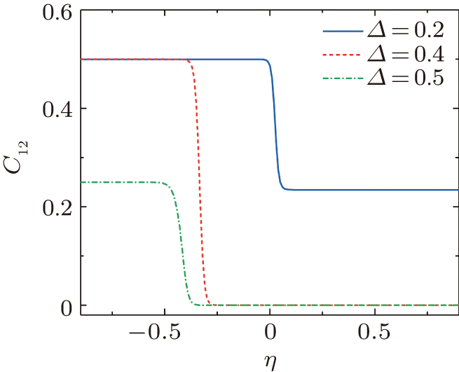
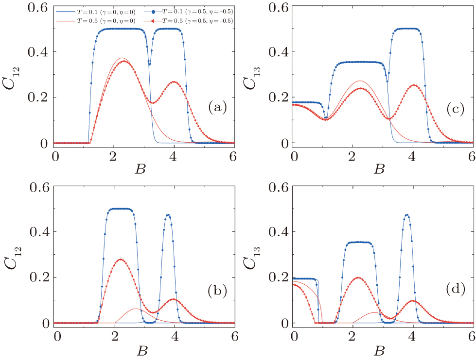
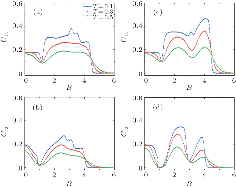
Abstract We investigate the effect of impurities on the thermal entanglement in a spin-1/2 Ising–Heisenberg butterfly-shaped chain, where four interstitial Heisenberg spins are localized on the vertices of a rectangular plaquette in a unit block. By using the transfer-matrix approach, we numerically calculate the partition function and the reduced density matrix of this model. The bipartite thermal entanglement between different Heisenberg spin pairs is quantified by the concurrence. We also discuss the fluctuations caused by the impurities through the uniform distribution and the Gaussian distribution. Considering the effects of the external magnetic field, temperature, Heisenberg and Ising interactions as well as the parameter of anisotropy on the thermal entanglement, our results show that comparing with the case of the clean model, in both the two-impurity model and the impurity fluctuation model the entanglement is more robust within a certain range of anisotropic parameters and the region of the magnetic field where the entanglement occurred is also larger.
|
Received: 13 August 2020
Revised: 01 September 2020
Accepted manuscript online: 01 January 1900
|
| Fund: the National Natural Science Foundation of China (Grant No. 12074101), the Science Fund for the New Century Excellent Talents in University of the Ministry of Education of China (Grant No. NCET-11-0960), and the Specialized Research Fund for the Doctoral Program of Higher Education of China (Grant No. 20134208110001). |
|
Corresponding Authors:
†Corresponding author. E-mail: maozhu@hubu.edu.cn ‡Corresponding author. E-mail: binzhou@hubu.edu.cn
|
Cite this article:
Meng-Ru Ma(马梦如), Yi-Dan Zheng(郑一丹), Zhu Mao(毛竹), and Bin Zhou(周斌) Thermal entanglement in a spin-1/2 Ising–Heisenberg butterfly-shaped chain with impurities 2020 Chin. Phys. B 29 110308
|
| [1] |
Bell J S 1987 Speakable and unspeakable in quantum mechanics Cambridge Cambridge University
|
| [2] |
Peres A 2006 Quantum theory: concepts and methods Springer Science & Business Media
|
| [3] |
|
| [4] |
|
| [5] |
|
| [6] |
|
| [7] |
|
| [8] |
|
| [9] |
|
| [10] |
|
| [11] |
|
| [12] |
|
| [13] |
|
| [14] |
|
| [15] |
|
| [16] |
|
| [17] |
|
| [18] |
|
| [19] |
|
| [20] |
|
| [21] |
|
| [22] |
|
| [23] |
|
| [24] |
|
| [25] |
Baxter R J 1982 Exactly solved models in statistical mechanics New York Academic Press
|
| [26] |
Yeomans J M 1992 Statistical mechanics of phase transitions Clarendon Press
|
| [27] |
|
| [28] |
|
| [29] |
|
| [30] |
|
| [31] |
|
| [32] |
|
| [33] |
|
| [34] |
Rule K C Reehuis M Gibson M C R Ouladdiaf B Gutmann M J Hoffmann J U Gerischer S Tennant D A Süllow S Lang M 2011 Phys. Rev. B 83 104401 DOI: 10.1103/PhysRevB.83.104401 |
| [35] |
Jeschke H Opahle I Kandpal H Valentí R Das H Saha-Dasgupta T Janson O Rosner H Brühl A Wolf B Lang M Richter J Hu S Wang X Peters R Pruschke T Honecker A 2011 Phys. Rev. Lett. 106 217201 DOI: 10.1103/PhysRevLett.106.217201 |
| [36] |
|
| [37] |
|
| [38] |
|
| [39] |
|
| [40] |
|
| [41] |
|
| [42] |
|
| [43] |
|
| [44] |
|
| [45] |
|
| [46] |
|
| [47] |
|
| No Suggested Reading articles found! |
|
|
Viewed |
|
|
|
Full text
|
|
|
|
|
Abstract
|
|
|
|
|
Cited |
|
|
|
|
Altmetric
|
|
blogs
Facebook pages
Wikipedia page
Google+ users
|
Online attention
Altmetric calculates a score based on the online attention an article receives. Each coloured thread in the circle represents a different type of online attention. The number in the centre is the Altmetric score. Social media and mainstream news media are the main sources that calculate the score. Reference managers such as Mendeley are also tracked but do not contribute to the score. Older articles often score higher because they have had more time to get noticed. To account for this, Altmetric has included the context data for other articles of a similar age.
View more on Altmetrics
|
|
|