|
Special Issue:
SPECIAL TOPIC — Machine learning in condensed matter physics
|
|
|
|
Machine learning identification of impurities in the STM images |
| Ce Wang(王策)1, Haiwei Li(李海威)2, Zhenqi Hao(郝镇齐)2, Xintong Li(李昕彤)2, Changwei Zou(邹昌炜)2, Peng Cai(蔡鹏)3, †, Yayu Wang(王亚愚)2,4, Yi-Zhuang You(尤亦庄)5,, ‡, and Hui Zhai(翟荟)1,§ |
1 Institute for Advanced Study, Tsinghua University, Beijing 100084, China
2 State Key Laboratory of Low Dimensional Quantum Physics, Department of Physics, Tsinghua University, Beijing 100084, China
3 Department of Physics and Beijing Key Laboratory of Opto-electronic Functional Materials and Micro-nano Devices, Renmin University of China, Beijing 100872, China
4 Frontier Science Center for Quantum Information, Beijing 100084, China
5 Department of Physics, University of California, San Diego, California 92093, USA |
|
|
|
|
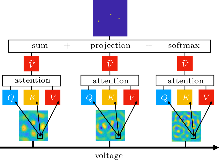
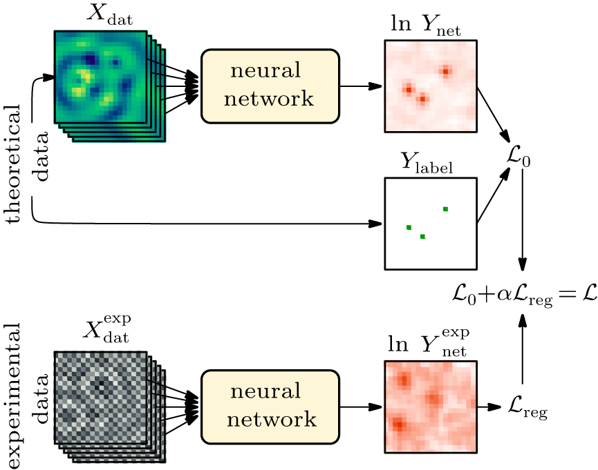
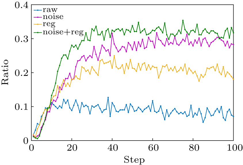
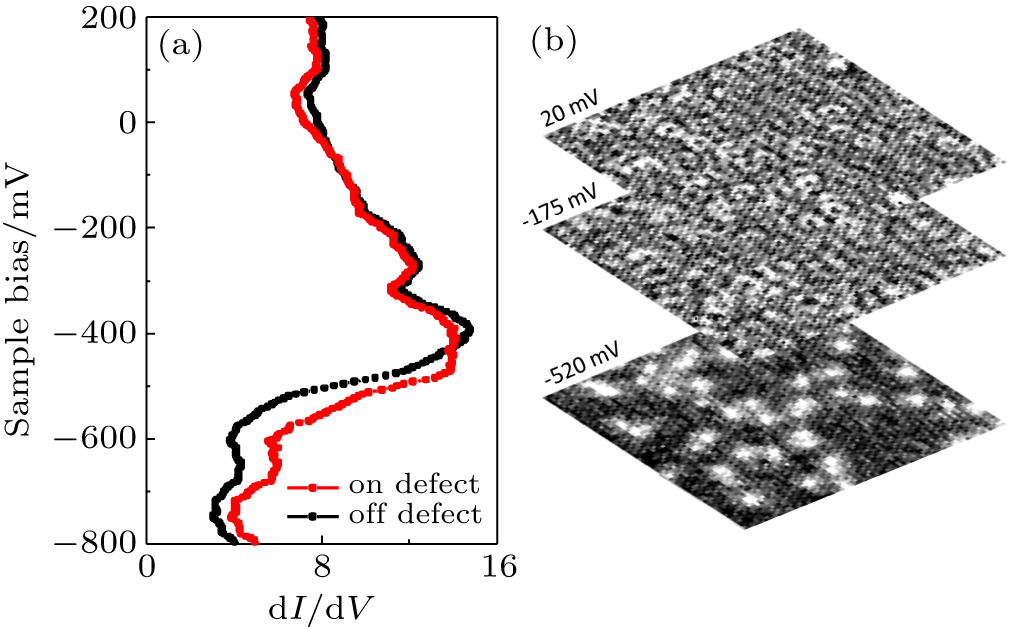
Abstract We train a neural network to identify impurities in the experimental images obtained by the scanning tunneling microscope (STM) measurements. The neural network is first trained with a large number of simulated data and then the trained neural network is applied to identify a set of experimental images taken at different voltages. We use the convolutional neural network to extract features from the images and also implement the attention mechanism to capture the correlations between images taken at different voltages. We note that the simulated data can capture the universal Friedel oscillation but cannot properly describe the non-universal physics short-range physics nearby an impurity, as well as noises in the experimental data. And we emphasize that the key of this approach is to properly deal with these differences between simulated data and experimental data. Here we show that even by including uncorrelated white noises in the simulated data, the performance of the neural network on experimental data can be significantly improved. To prevent the neural network from learning unphysical short-range physics, we also develop another method to evaluate the confidence of the neural network prediction on experimental data and to add this confidence measure into the loss function. We show that adding such an extra loss function can also improve the performance on experimental data. Our research can inspire future similar applications of machine learning on experimental data analysis.
|
Received: 02 July 2020
Revised: 07 August 2020
Accepted manuscript online: 14 October 2020
|
| Fund: HZ is supported by Beijing Outstanding Scholar Program, the National Key Research and Development Program of China (Grant No. 2016YFA0301600), and the National Natural Science Foundation of China (Grant No. 11734010). YZY is supported by a startup fund from UCSD. PC is supported by the Fundamental Research Funds for the Central Universities, and the Research Funds of Renmin University of China. |
|
Corresponding Authors:
†Corresponding author. E-mail: pcai@ruc.edu.cn ‡Corresponding author. E-mail: yzyou@ucsd.edu §Corresponding author. E-mail:hzhai@tsinghua.edu.cn
|
Cite this article:
Ce Wang(王策), Haiwei Li(李海威), Zhenqi Hao(郝镇齐), Xintong Li(李昕彤), Changwei Zou(邹昌炜), Peng Cai(蔡鹏), Yayu Wang(王亚愚), Yi-Zhuang You(尤亦庄), and Hui Zhai(翟荟) Machine learning identification of impurities in the STM images 2020 Chin. Phys. B 29 116805
|
| [1] |
|
| [2] |
Torlai G, Timar B, van Nieuwenburg E P L, Harry L, Omran A, Keesling A, Bernien H, Greiner M, Vuletić V, Lukin M D, Melko R G, Endres M 2019 Phys. Rev. Lett. 123 230504 DOI: 10.1103/PhysRevLett.123.230504 |
| [3] |
Zhang Y, Mesaros A, Fujita K, Edkins SD, Hamidian MH, Ch’ng K, Eisaki H, Uchida S, Davis JCS, Khatami E, Kim EA 2019 Nature 570 484 DOI: 10.1038/s41586-019-1319-8 |
| [4] |
Rem B S, Käming N, Tarnowski M, Asteria L, Fläschner N, Becker C, Sengstock K, Weitenberg C 2019 Nat. Phys. 15 917 DOI: 10.1038/s41567-019-0554-0 |
| [5] |
Bohrdt A, Chiu C S, Ji G, Xu M, Greif D, Greiner M, Demler E, Grusdt F, Knap M 2019 Nat. Phys. 15 921 DOI: 10.1038/s41567-019-0565-x |
| [6] |
Samarakoon A M, Barros K, Li Y W, Eisenbach M, Zhang Q, Ye F, Dun Z L, Zhou H, Grigera S A, Batista C D, Tennant D A 2020 Nat. Commun. 11 892 DOI: 10.1038/s41467-020-14660-y |
| [7] |
Khatami E, Guardado-Sanchez E, Spar B M, Carrasquilla J F, Bakr W S, Scalettar R T 2020 arXiv: 2002.12310 [cond-mat.str-el] |
| [8] |
Bishop C M 2006 Pattern recognition and machine learning New York Springer 592 595
|
| [9] |
Vaswani A, Shazeer N, Parmar N, Uszkoreit J, Jones L, Gomez A N, Kaiser L, Polosukhin I 2017 arXiv: 1706.03762 [cs.CL] |
| [10] |
Devlin J, Chang M W, Lee K, Toutanova K 2018 arXiv: 1810.04805 [cs.CL] |
| [11] |
|
| No Suggested Reading articles found! |
|
|
Viewed |
|
|
|
Full text
|
|
|
|
|
Abstract
|
|
|
|
|
Cited |
|
|
|
|
Altmetric
|
|
blogs
Facebook pages
Wikipedia page
Google+ users
|
Online attention
Altmetric calculates a score based on the online attention an article receives. Each coloured thread in the circle represents a different type of online attention. The number in the centre is the Altmetric score. Social media and mainstream news media are the main sources that calculate the score. Reference managers such as Mendeley are also tracked but do not contribute to the score. Older articles often score higher because they have had more time to get noticed. To account for this, Altmetric has included the context data for other articles of a similar age.
View more on Altmetrics
|
|
|