|
|
|
Nonlinear dynamics of a classical rotating pendulum system with multiple excitations |
| Ning Han(韩宁)† and Pei-Pei Lu(鲁佩佩) |
| Key Laboratory of Machine Learning and Computational Intelligence, College of Mathematics and Information Science, Hebei University, Baoding 071002, China |
|
|
|
|
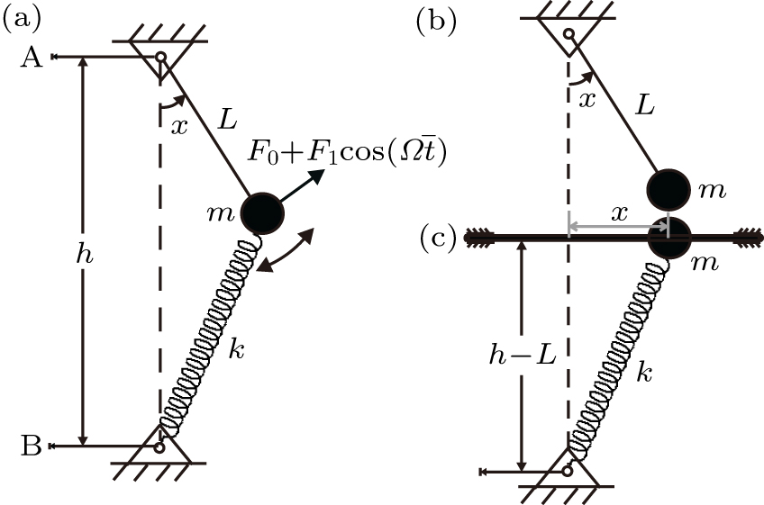
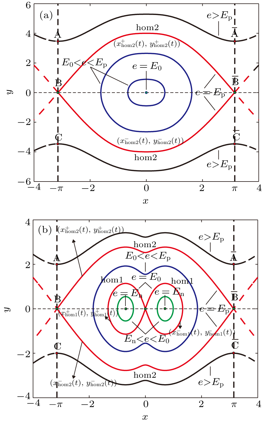
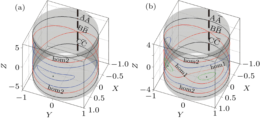
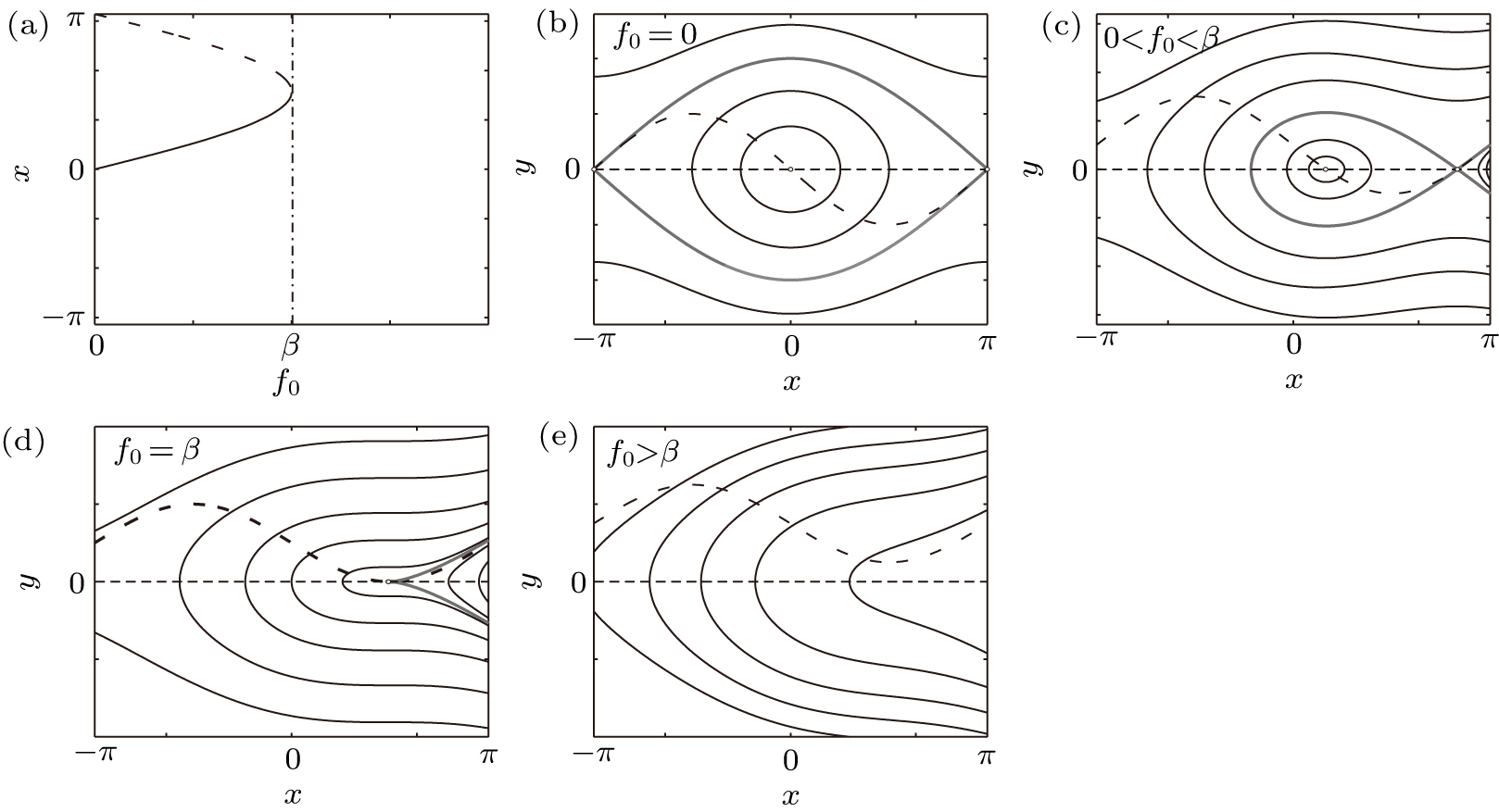
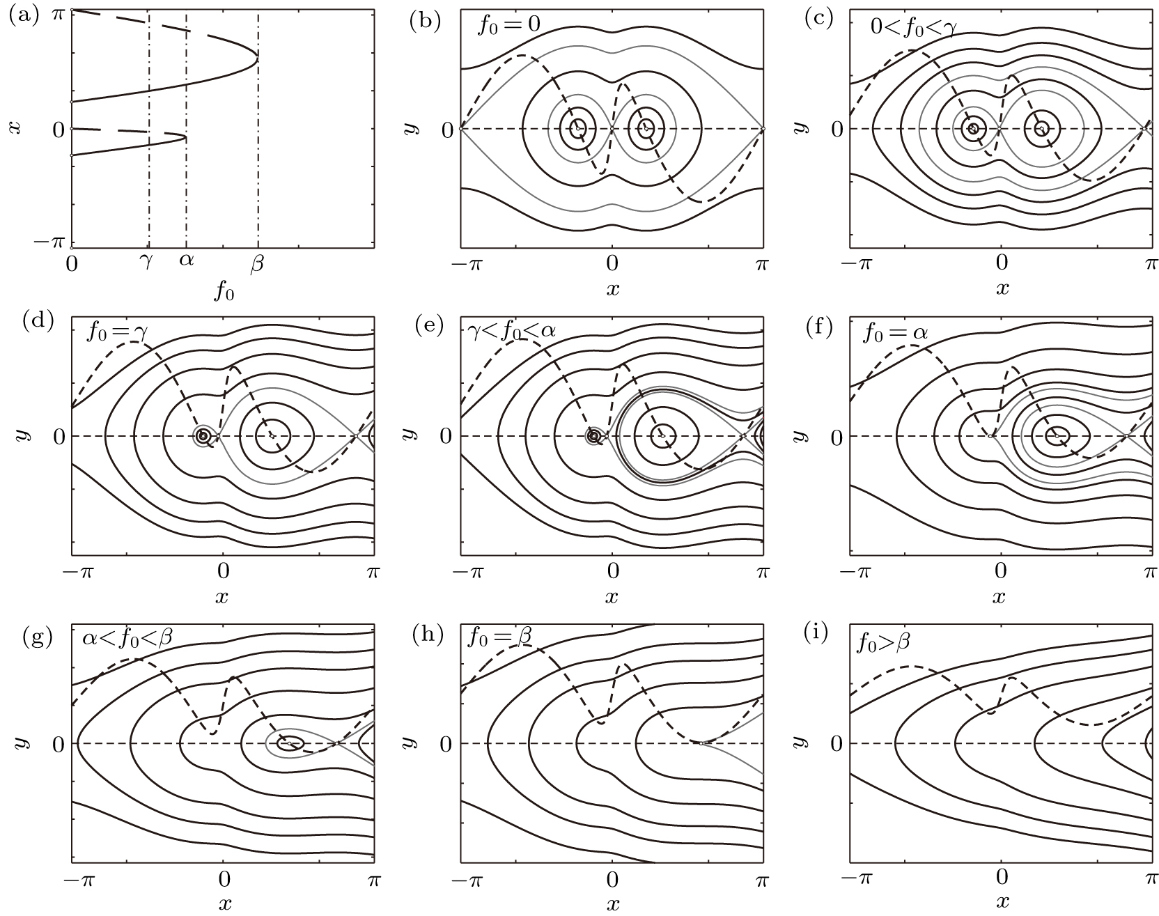
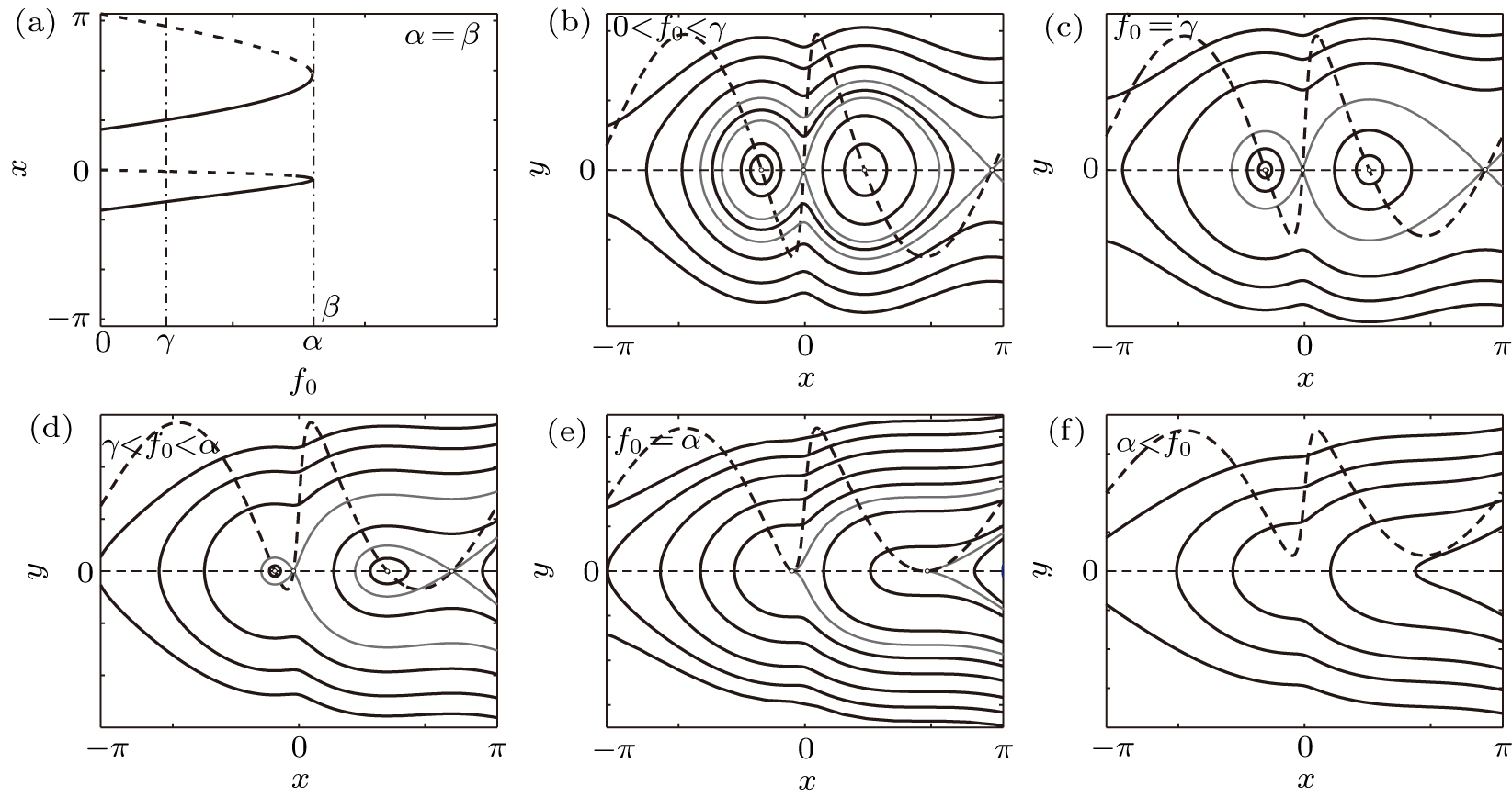
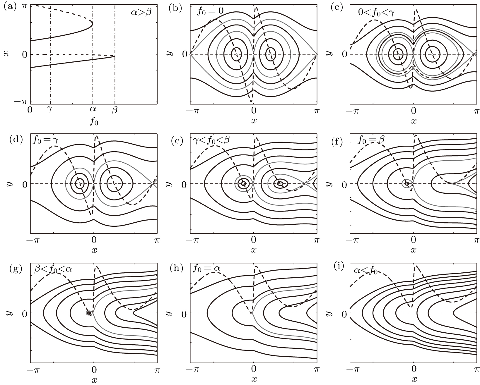
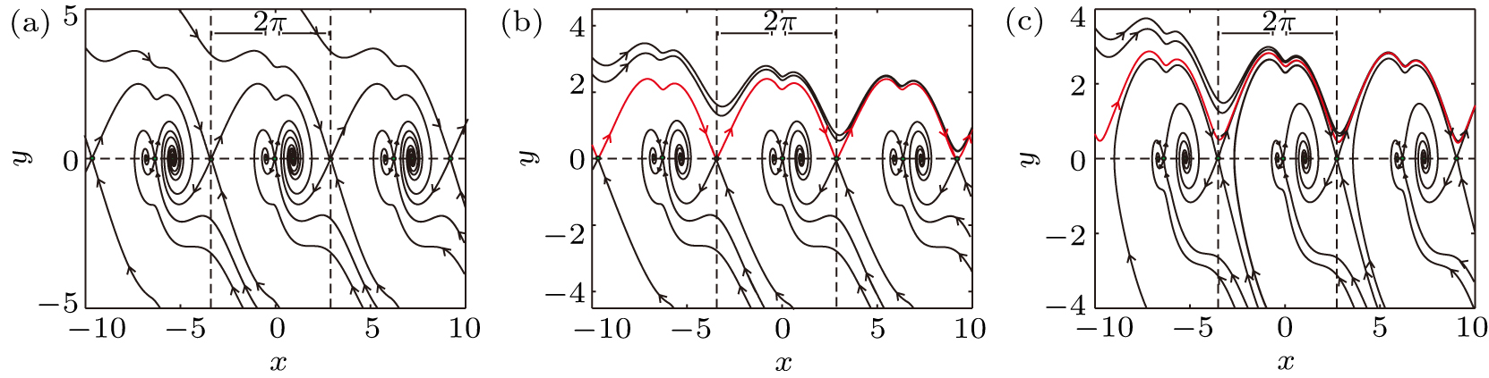
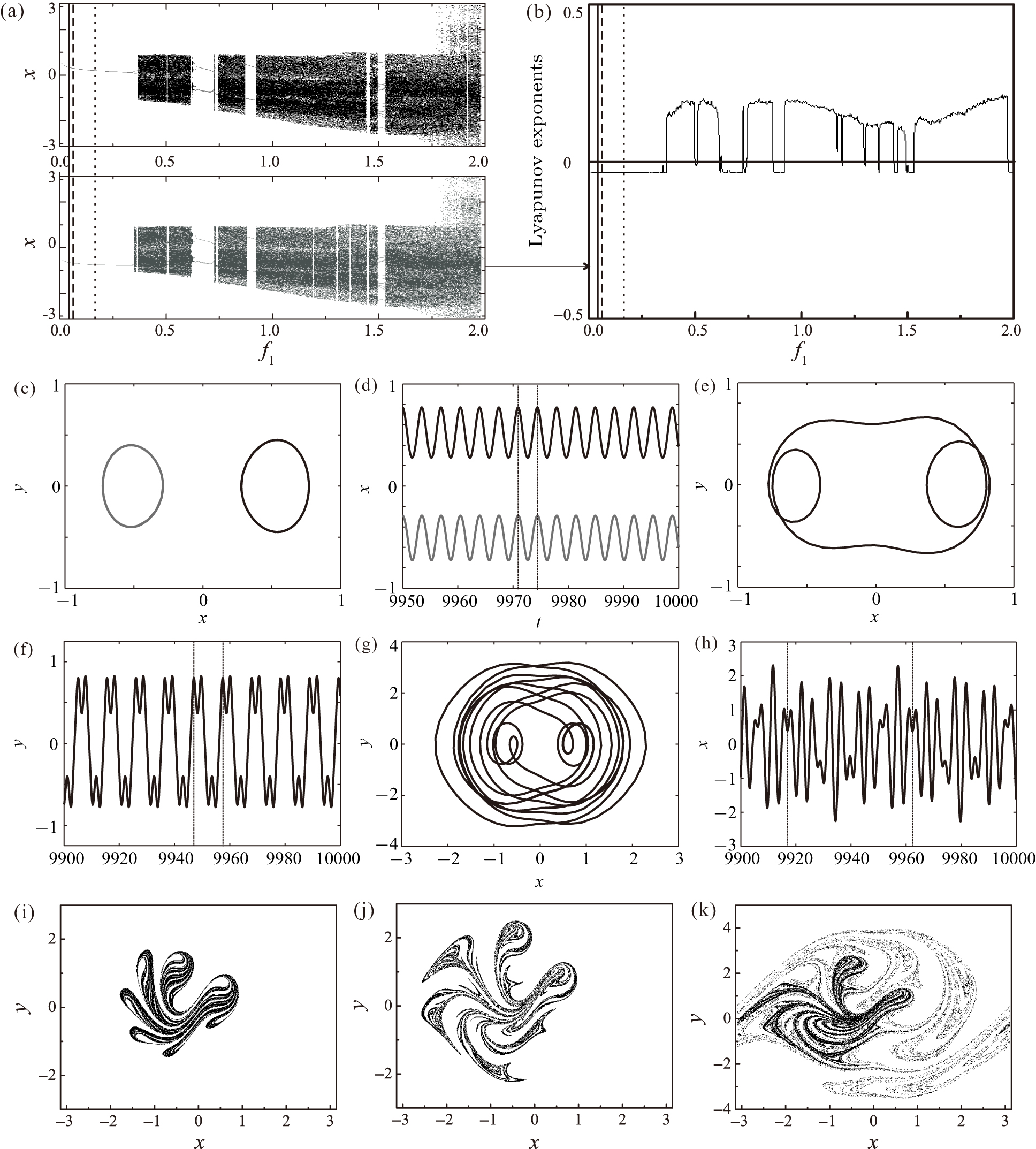
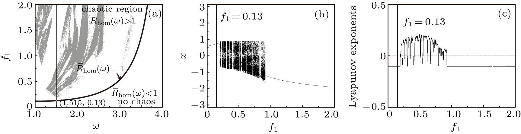
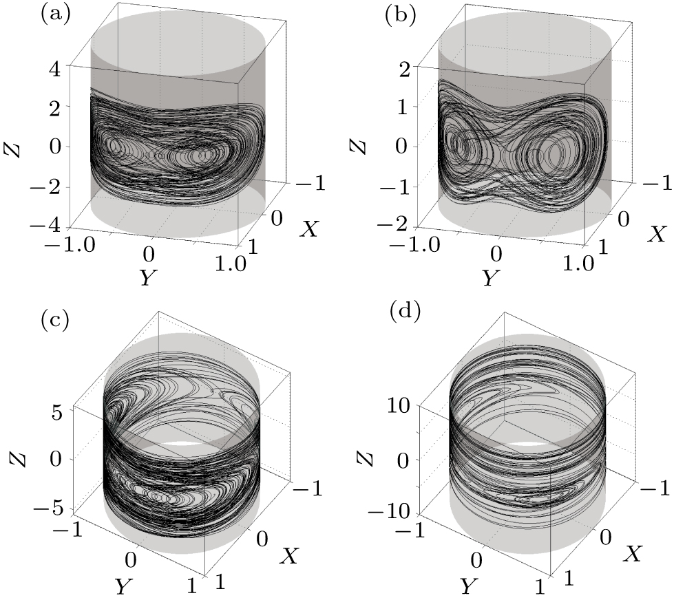
Abstract We report an attempt to reveal the nonlinear dynamic behavior of a classical rotating pendulum system subjected to combined excitations of constant force and periodic excitation. The unperturbed system characterized by strong irrational nonlinearity bears significant similarities to the coupling of a simple pendulum and a smooth and discontinuous (SD) oscillator, especially the phase trajectory with coexistence of Duffing-type and pendulum-type homoclinic orbits. In order to learn the effect of constant force on this pendulum system, all types of phase portraits are displayed by means of the Hamiltonian function with large constant excitation especially the transitions of complex singular closed orbits. Under sufficiently small perturbations of the viscous damping and constant excitation, the Melnikov method is used to analyze the global structure of the phase space and the feature of trajectories. It is shown, both theoretically and numerically, that this system undergoes a homoclinic bifurcation and then bifurcates a unique attracting rotating limit cycle. Finally, the estimation of the chaotic threshold of the rotating pendulum system with multiple excitations is calculated and the predicted periodic and chaotic motions can be shown by applying numerical simulations.
|
Received: 06 April 2020
Revised: 09 June 2020
Accepted manuscript online: 18 June 2020
|
| Fund: the National Natural Science Foundation of China (Grant Nos. 11702078 and 11771115), the Natural Science Foundation of Hebei Province, China (Grant No. A2018201227) and the High-Level Talent Introduction Project of Hebei University, China (Grant No. 801260201111). |
|
Corresponding Authors:
†Corresponding author. E-mail: hanning.bing@163.com; ninghan@hbu.edu.cn
|
Cite this article:
Ning Han(韩宁) and Pei-Pei Lu(鲁佩佩) Nonlinear dynamics of a classical rotating pendulum system with multiple excitations 2020 Chin. Phys. B 29 110502
|
| [1] |
|
| [2] |
Matthews M R, Gauld C F, Stinner A 2005 The Pendulum: Scientific, Historical, Philosophical and Educational Perspectives Dordrecht Springer 139
|
| [3] |
|
| [4] |
|
| [5] |
|
| [6] |
|
| [7] |
|
| [8] |
|
| [9] |
|
| [10] |
|
| [11] |
|
| [12] |
|
| [13] |
|
| [14] |
|
| [15] |
|
| [16] |
|
| [17] |
|
| [18] |
|
| [19] |
|
| [20] |
|
| [21] |
|
| [22] |
|
| [23] |
|
| [24] |
|
| [25] |
|
| [26] |
|
| [27] |
Jia M M, Jiang H G, Li W J 2019 Acta Phys. Sin. 68 130503 in Chinese
|
| [28] |
Cao Q J, Han N, Tian R L 2011 Chin. Phys. Lett. 28 0605021
|
| [29] |
|
| [30] |
Han N, Cao Q J 2016 Commun. Nonlinear Sci. Numer. Simulat. 36 431
|
| [31] |
|
| [32] |
|
| [33] |
Hong L, Xu J 2004 Commun. Nonlinear Sci. Numer. Simulat. 9 313
|
| [34] |
|
| [35] |
|
| [36] |
|
| [37] |
|
| [38] |
Cao Q J, Wiercigroch M, Pavlovskaia E E, Grebogi C, Thompson J M T 2008 Philos. Trans. R. Soc. A 366 635 DOI: 10.1098/rsta.2007.2115 |
| [39] |
Guckenheimer J, Holmes P 1983 Nonlinear Oscillations, Dynamical Systems, and Bifurcations of Vector Fields New York Springer 184
|
| [40] |
Melnikov V K 1963 Trans. Moscow. Math. Soc. 12 1
|
| [41] |
Hu H Y 2000 Applied Nonlinear Dynamics Beijing Aviation Industry Press of China 38 in Chinese
|
| [42] |
Strogatz S H 2015 Nonlinear Dynamics and Chaos: With Applications to Physics, Biology, Chemistry, and Engineering Beijing China Machine Press 272
|
| [43] |
|
| [44] |
|
| [45] |
|
| [46] |
|
| [47] |
Albert Luo C J 2017 Resonance and Bifurcation to Chaos in Pendulum Beijing Higher Education Press of China 220
|
| [48] |
Liu Y Z, Chen L Q 2001 Nonlinear Vibrations Beijing Aviation Industry Press of China 286 in Chinese
|
| [49] |
Feng J Q 2018 Nonlinear Dynamics of a Typical Vibro-Impact System Beijing Science Press of China 95 in Chinese
|
| No Suggested Reading articles found! |
|
|
Viewed |
|
|
|
Full text
|
|
|
|
|
Abstract
|
|
|
|
|
Cited |
|
|
|
|
Altmetric
|
|
blogs
Facebook pages
Wikipedia page
Google+ users
|
Online attention
Altmetric calculates a score based on the online attention an article receives. Each coloured thread in the circle represents a different type of online attention. The number in the centre is the Altmetric score. Social media and mainstream news media are the main sources that calculate the score. Reference managers such as Mendeley are also tracked but do not contribute to the score. Older articles often score higher because they have had more time to get noticed. To account for this, Altmetric has included the context data for other articles of a similar age.
View more on Altmetrics
|
|
|