
Enhancement of photoacoustic tomography in the tissue with speed-of-sound variance using ultrasound computed tomography*
[Cheng Ren-Xiang, Tao Chao , Liu Xiao-Jun]
, Liu Xiao-Jun]
|
|


†Corresponding author. E-mail: taochao@nju.edu.cn
Corresponding author. E-mail: liuxiaojun@nju.edu.cn
*Projection supported by the National Basic Research Program of China (Grant No. 2012CB921504), the National Natural Science Foundation of China (Grant Nos. 11422439, 11274167, and 11274171), and the Specialized Research Fund for the Doctoral Program of Higher Education, China (Grant No. 20120091110001).
The speed-of-sound variance will decrease the imaging quality of photoacoustic tomography in acoustically inhomogeneous tissue. In this study, ultrasound computed tomography is combined with photoacoustic tomography to enhance the photoacoustic tomography in this situation. The speed-of-sound information is recovered by ultrasound computed tomography. Then, an improved delay-and-sum method is used to reconstruct the image from the photoacoustic signals. The simulation results validate that the proposed method can obtain a better photoacoustic tomography than the conventional method when the speed-of-sound variance is increased. In addition, the influences of the speed-of-sound variance and the fan-angle on the image quality are quantitatively explored to optimize the image scheme. The proposed method has a good performance even when the speed-of-sound variance reaches 14.2%. Furthermore, an optimized fan angle is revealed, which can keep the good image quality with a low cost of hardware. This study has a potential value in extending the biomedical application of photoacoustic tomography.
Photoacoustic tomography (PAT)[1] is a fast-growing medical imaging technology, which combines the rich optical contrast with the high ultrasonic resolution in deep tissue. Optical contrasts are closely associated with the physiological function of the tissue. However, strong optical scattering restricts the spatial resolution of the pure optical imaging method in deep tissue.[2] Acoustic scattering in the tissue is two to three orders of magnitude less than light scattering, which makes ultrasound (US) effectively focus in deep tissue. Hybridizing optical contrast and photoacoustic (PA) detection, PAT can sensitively reveal the functional and structural information of deep tissue with an acoustically spatial resolution. Besides, non-ionizing radiation, e.g., laser and microwave, used in PAT is much safer than the ionizing radiation, e.g., x-ray. These merits make PAT have a great prospect in biomedical applications, such as detecting breast cancer, [3] brain imaging, [4, 5] vessel disease detection, [6, 7] etc.[8– 16]
Generally, PAT is suitable for the tissue with inhomogeneous optical absorption and homogeneous acoustic properties. The inhomogeneous optical absorption promises a good image contrast. The homogeneousness of the acoustic properties makes it easy to accurately calculate the time-of-flight (TOF) of PA waves.[17] Many PAT applications have assumed that the biological tissue in the entire region of interest (ROI) is acoustically homogeneous and has a constant speed of sound (SOS).[18] However, the SOS of the real tissue is inhomogeneous. The SOS could be changed from 1400 m/s in the fat to 1600 m/s in the musculature.[19, 20] When reconstructing the PAT images, the discrepancies of the SOS will result in calculation deviation of TOF. This deviation leads to image blurring, distortion, and even prevents getting distinguishable images.[21– 23]
Some studies have been done to improve the image quality in the tissue with SOS variance. Treeby et al. presented an autofocus approach to automatically select the SOS by maximizing the sharpness of the reconstructed image.[24] Deá n-Ben et al. proposed a statistical reconstruction method to improve the image quality and quantification by using a priori knowledge on the location of the acoustic distortions.[25, 26] Jiang et al.[27] and Yuan et al.[28] developed a finite-element reconstruction algorithm for the simultaneous reconstruction of both optical and acoustic properties of heterogeneous media. Manohar et al.[29] and Jose et al.[23– 30] presented a method based on the photoacoustic principle to recover the light absorption, SOS distribution, and acoustic attenuation in the tissue. Li et al. proposed a linear-delay-compensation based reconstruction approach to focus the whole PAT image region for an SOS heterogeneous tissue.[31] Zhang and Wang proposed an inverse reconstruction algorithm by utilizing the correlation information of PA signals to compensate for the acoustic heterogeneity.[32] Jin and Wang, [33] Xia et al., [34] and Huang et al.[35] developed a full-wave method to iterative image reconstruction in PAT, which was based on the exact PA wave equation in inhomogeneous acoustically media. However, the SOS variance is still a limitation to PAT applications.
In this paper, we combine ultrasound computed tomography (US-CT) with PAT to improve the PAT imaging quality in the acoustically inhomogeneous tissue. In this method, the devices of US-CT and PAT share the same US transducers. The SOS distribution information is restored by using US-CT. Then, according to the restored SOS distribution, an improved delay-and-sum (DAS) algorithm is proposed to enhance the PA images in the tissue with SOS distribution information. Numerical simulations are employed to examine the validation of the proposed method. Finally, in order to optimize the image scheme, we quantitatively explore the influences of the SOS variance and fan angle on the image quality.
Our basic idea is to combine the ability of US-CT in SOS imaging with PAT. US-CT extracts the SOS information in the ROI. Then, the obtained SOS information is employed to improve the quality of the PAT image. Here, the US pulse is assumed to travel along a straight line through the media, namely, the US refraction effect is neglected or only weak US refraction exists in the tissue.[33]
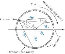
The imaging system is shown in Fig. 1. A ring US transducer array is arranged at the closed curve surrounding the imaging region. The US transducer array is used for both the US-CT procedure and the PAT procedure.
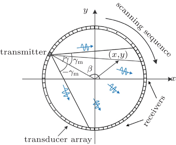 | Fig. 1. Schematic of scanning geometry. A US transducer element at angular position β is used as the transmitter to launch US pulses. The other elements on the opposite side of the transmitter are used as the receivers to detect the US pulses. The process is repeated to make the fan-beam (light gray region) rotate 360 degrees around the tissue. |
First, an US-CT method is used to determine the SOS distribution in the ROI. An US transmitting-receiving system is employed to acquire the propagation time of the US pulse in the acoustically inhomogeneous tissue. During this process, an US transducer element at angular position β is used as the transmitter to launch US pulses. The other elements of the US transducer array on the opposite side of the transmitter are used as the receivers to detect the US pulses. The transmitter and the receivers form a fan-beam with a fan angle 2γ m, as shown in Fig. 1. Angle γ gives the relative angular position of an US pulse propagation path taken at angle β . Therefore, the US pulse propagation path is uniquely determined by (β , γ ).
The above transmitting-receiving process is repeated for the elements in the transducer array one by one. The fan-beam (light gray region) will rotate 360 degree around the tissue. Totally, NProj US transducers in the US transducer array are chosen and used as the transmitters. The positions of the transmitters surround the specimen uniformly. An US pulse is launched from the transmitter and detected by the receivers on the opposite side of each transmitter. The US pulses are launched NProj times. The above process is completed, respectively, before and after the specimen is inserted.
After the US pulse passes through the tissue, its propagation time in the corresponding path is calculated. Before the specimen is inserted, the US pulse propagation time in corresponding path (β , γ ) is acquired and recorded as 
 |
Since the change of the US pulse propagation time is due to the SOS difference in the propagation path (β , γ ), we have the following relationship between the measured time difference R[β , γ ] and the SOS distribution:
 |
where v is the SOS distribution in the tissue, v0 is the SOS in the couple agent surrounding the specimen, and (β , γ ) represents the US pulse propagation path. The SOS distribution v can be obtained by solving Eq. (2) with the measured R[β , γ ].
The following algorithm[36, 37] is used to reconstruct the SOS distribution function. For an arbitrary imaging position (x, y) in the ROI, the US pulse propagation path (β n, γ n) that goes through (x, y) in the n-th transmitting-receiving process can be found. The corresponding time difference is recorded as R[β n, γ n]. Then, we have the average time difference of the US propagation path passing through the position (x, y)
 |
The SOS distribution at (x, y) can be estimated by
 |
The constant R0 is related to the specimen size and transducer spacing.[36, 37]
Second, PA signals are generated. Using the generated PA signals and the SOS information provided by US-CT, a CT-corrected delay-and-sum (CT-Corrected DAS) method is proposed to reconstruct the PA images. We keep the position of the specimen and use a pulse laser to irradiate the ROI. The same US transducer array is used to record the PA signals from the specimen. The received PA signals and the SOS distribution information are used to reconstruct the PA images
 |
Here, S(x, y) represents the relative optical absorption properties in the imaging region, wk(x, y) is the weighting factor, which takes into account the angular sensitivity of detector k, Pk(Tk) is the PA signal received by detector k, and Tk is TOF from spatial position (x, y) to detector k along a straight path. The Tk is calculated by
 |
where v(x, y) is the SOS distribution determined by the US-CT in the first step. It is noticed that if v(x, y) is replaced by a constant in Eq. (6), equation (5) will degenerate to the commonly used DAS algorithm.
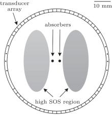
Numerical experiments are carried out to examine the validation of the proposed method. Figure 2 illustrates the setup of the numerical experiments. The US transducer array is arranged along the circle with a radius of 30 mm enclosing the ROI. Two dark-gray dots represent the optical absorbers with a radius of 1.3 mm. The optical absorbers have SOS of 1400 m/s and density of 1.0 g/cm3, which are the same as the surrounding media (white region). Two light gray ellipses are acting as the high SOS region. The elliptical long axis is 38 mm and the elliptical short axis is 16 mm. Their density is 1.0 g/cm3, which are the same as the surrounding media. However, their SOS is higher than the surrounding tissue. The relative optical absorption intensity of the absorbers is 1.0, while that of the other regions is 0.0.
US pulses with a central frequency of 0.5 MHz are launched for the SOS estimation. The mesh size is 0.5 mm. The US pulses are received by the receivers. The sampling frequency is 20 MHz, and the SOS distribution is restored by using Eqs. (3) and (4). Then, a Gaussian pulse with a central frequency of 2.5 MHz is emitted by the absorbers, which simulates the generation of the PA signals. The mesh size is 0.18 mm. The PA signals are detected by the same US transducer array used in the US-CT process. The size of the ROI is 40 mm× 40 mm, and the center of the ROI is overlapped with the center of the transducer array. The sampling frequency is 20 MHz. The numerical simulation is executed by using the acoustic module in commercial finite-element software COMSOL.
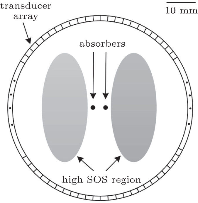 | Fig. 2. Diagram of simulation setup. The dark gray dots are optical absorbers and light gray ellipses are the high SOS region. The US transducer array surrounded the specimen is used in both processes of US-CT and photoacoustic imaging. |
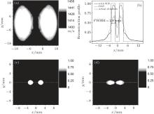
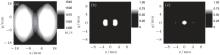
Figure 3 gives the simulation results with NProj = 90 and fan angle 2γ m = 90° , where the SOS of the high SOS region is 1455 m/s. Figure 3(a) shows the SOS distribution recovered by the US-CT according to Eqs. (3) and (4). It is seen that the reconstructed SOS distribution well matches the real SOS distribution in the ROI. Two high SOS regions are clearly identified. Using the estimated SOS distribution, the PA image is reconstructed from the detected PA signals. As shown in Fig. 3(c), the position and size of the absorbers in the image are consistent with the actual situation. For comparison, the PA image is also reconstructed by using the DAS method, where a homogeneous SOS of 1400 m/s is assumed in the tissue. As shown in Fig. 3(d), the lack of the SOS information results in a blurred image of the absorbers. The reconstructed image of the absorbers is seriously deformed and its size is far from the actual situation. Figure 3(b) compares the reconstructed profiles along the cross section at y = 0 (the dash lines in Figs. 3(c) and 3(d)). As shown, the SOS inhomogeneousness induces a distortion in the image reconstructed with DAS. However, the image obtained by the CT-corrected DAS is still close to the actual situation. These preliminary simulations validate that the proposed PAT method can effectively improve the image quality of the tissue with inhomogeneous SOS.
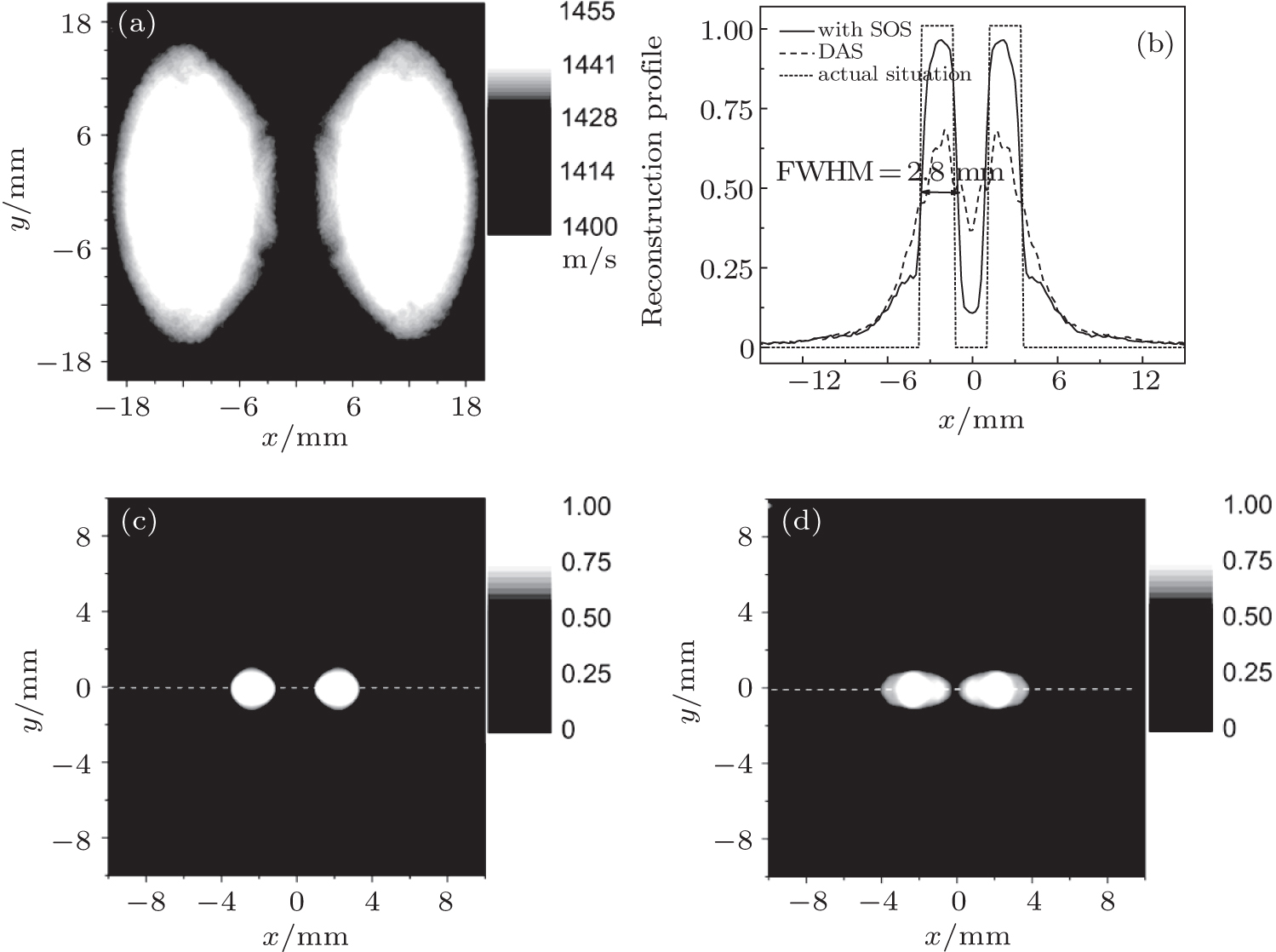 | Fig. 3. Comparison of PAT reconstruction by using the proposed method and the DAS method. The SOS of the high SOS region is 1455 m/s. (a) The SOS distribution estimated by US-CT. (b) The profile of image intensity along the cross section at y = 0 (the dotted lines in panels (c) and (d)). The short dash line is the actual profile. The solid line and the dash dashed line are the reconstructed profiles with the proposed method and DAS, respectively. (c) The reconstructed PAT image by the CT-corrected DAS. (d) The reconstructed PAT image by DAS. |
Generally, the weak refraction assumption is one important precondition of US-CT. Under this condition, it can be approximately considered that the US pulses propagate along a straight line. This assumption would limit the US-CT and the proposed PAT scheme to the situation of a small variation of SOS. When the variation of SOS is increased and the refraction effect is stronger, the precondition is broken, and the accuracy of the SOS estimation and the PAT image quality are reduced. Therefore, it will be necessary to examine the effectiveness of the proposed PAT scheme when the variation of SOS is large.
Numerical simulations are carried out to examine the relationship between the quality of the PA image and the variation degree of SOS. The SOS difference Δ v is defined to quantify the variation degree of the tissue SOS distribution
 |
where vh is the SOS of the high SOS region and v0 = 1400 m/s is the SOS of the surrounding media. A larger Δ v indicates the greater SOS variation and the stronger acoustic refraction. The image quality is quantified by the correlation coefficient rcorr defined as
 |
where the matrix A is the actual distribution of the optical absorbing properties in the ROI, the matrix B is the reconstructed PA image, cov(A, B) is the covariance of A and B, and σ A and σ B are the standard deviations of A and B, respectively. The correlation coefficient rcorr indicates the similarity between the actual and the reconstructed PA images. A larger rcorr illustrates a better quality of the reconstructed PA image. The same two images have a correlation coefficient rcorr = 1.
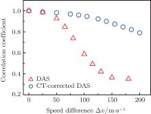
Figure 4 gives the relationship between the correlation coefficient rcorr and the SOS difference Δ v. As shown, the image quality is closely associated with the variation degree of SOS. When the SOS difference Δ v is tiny (Δ v < 30 m/s), both the DAS method and the proposed method can provide good images. The effect of the SOS inhomogeneousness can be neglected. With the increase of Δ v, the imaging qualities of DAS and CT-corrected DAS both decline. However, the image obtained by the CT-corrected DAS has a larger correlation coefficient than that obtained by DAS.
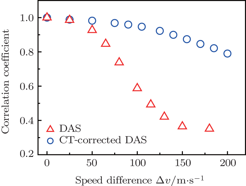 | Fig. 4. The effect of SOS difference Δ v on imaging quality. Here Δ v is defined as the speed difference between the high speed region and the surrounding tissue. The image quality is measured by the correlation coefficient. |
When Δ v is larger than 140 m/s, the PA image reconstructed by DAS shown in Fig. 5(c) is distorted so seriously that two absorbers cannot be distinguished in the image. The refraction effect also decreases the accuracy of the SOS distribution recovering, as shown in Fig. 5(a). However, the recovered SOS information is still a significant help to the imaging quality. Figure 5(b) shows the PA image reconstructed by CT-corrected DAS. It is seen that the reconstructed image is much better than that obtained by DAS. The positions of the absorbers are still consistent with the actual situation. The reconstruction results are acceptable.
 | Fig. 5. The images are reconstructed at Δ v = 140 m/s. (a) The SOS distribution obtained by US-CT. (b) and (c) PAT images obtained by the CT-corrected DAS and DAS directly. |
Generally, the increase of the SOS variance will lower the imaging quality of CT-corrected DAS. However, its quality is much better than that of the DAS method. Moreover, even when Δ v reaches 200 m/s (200/1400 × 100% ≈ 14.2%), the CT-corrected DAS can still obtain a distinguishable PA image. It is known that the SOS variance in the soft tissue is usually no more than 11%.[19] Therefore, although the proposed method is developed under the weak reflection assumption, it still has a good performance when the speed variance is less than 14.2%, which is competent for the soft tissue imaging.
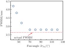
The fan angle 2γ m is another important factor that affects the accuracy of the SOS distribution estimation. Figure 6 illustrates the relationship between the quality of the reconstructed image and the fan angle 2γ m. The full width at half-maximum (FWHM) of the absorbers in the image is used to measure the imaging quality. Here, the FWMH is determined according to the profile along the cross section at y = 0, as shown in Fig. 3(b). In this simulation, the SOS of the high SOS region is 1455 m/s.
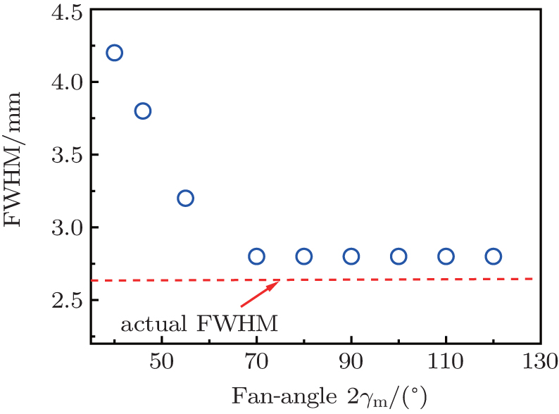 | Fig. 6. The relationship between the FWHM of the absorbers in the image and the fan-angle 2γ m. The dashed line illustrates the actual diameter 2.6 mm of the absorbers. The FWMH is determined according to the profile shown in Fig. 3(b). The SOS of the high SOS region is 1455 m/s. |
As shown, the imaging quality is closely associated with the fan angle. When the fan angle is small, the FWHM significantly deviates from the actual size 2.6 mm of the absorbers. The increase of the fan angle will make the FWHM approach to the diameter of the absorbers. Finally, when the fan angle is increased to 70° , the FWHM is about 2.8 mm, which is close to the actual diameter 2.6 mm. Beyond 70° , the increase of the fan angle will not continue to improve the image quality.
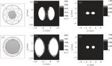
It can be explained as follows. When the fan angle is small, the calculation region covered by the US-CT is smaller than the inhomogeneous region, as shown in Fig. 7(a). In Figs. 7(a) and 7(d), the red dashed square represents the actual acoustically inhomogeneous region. The small calculation region makes the reconstructed SOS information not enough to reflect the actual situation of acoustic inhomogeneousness and the accuracy of the SOS estimation is reduced, as shown in Fig. 7(b). Furthermore, the low accuracy SOS information limits the quality of the PA image, as shown in Fig. 7(c). When the fan angle is sufficiently large, the calculation region of the US-CT will cover the whole inhomogeneous region (Fig. 7(d)). The accuracy of the SOS estimation is improved (Fig. 7(e)). The quality of the PA image (Fig. 7(f)) is enhanced with the accurate SOS information. When the fan angle is large enough to cover all inhomogeneous regions, further increase of the angle will not provide extra inhomogeneous SOS information. The image quality is no longer increased with the fan angle. The minimum fan angle, which can cover the whole acoustically inhomogeneous region, will be beneficial for improving the PAT quality and decreasing the cost of the system.
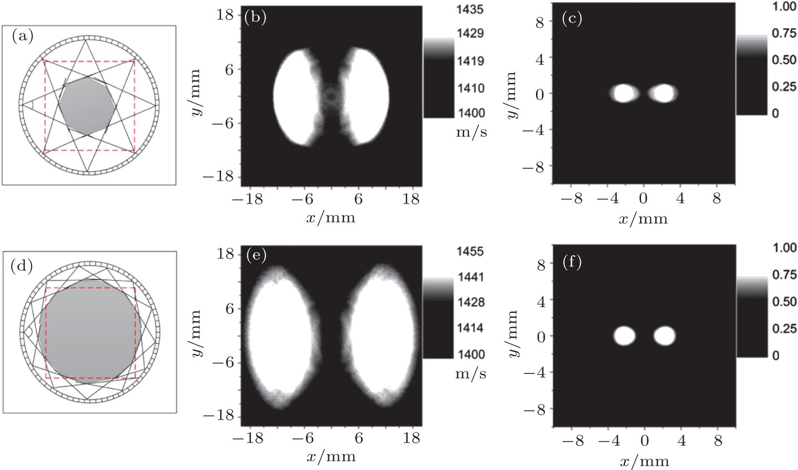 | Fig. 7. Comparison of reconstructed images in different fan angles. The upper row (a)– (c) and lower row (d)– (f) are reconstructed with fan angles 48° and 100° , respectively. The SOS of the high SOS region is 1455 m/s. The gray region in the left column is the region covered by US-CT. The red dashed square represents the acoustically inhomogeneous region. The middle columns are the recovered SOS distributions. The right columns are the reconstructed PA images. |
In the real situation, the SOS in the high SOS region may not be a constant, the measurement noise is inevitable, and the ultrasound transducer has a finite size. Figure 8 gives the simulation of a more realistic imaging process. As shown in Fig. 8(a), the SOS in the high SOS region is not a constant. The PA signals are spatially integrated over the transducer surface to simulate the PA signals detected by an US transducer with a finite diameter of 7 mm. Noise is added to the detected signals and the signal to noise ratio is 0.0 dB. Figure 8(b) gives the SOS distribution recovered by the US-CT. It is seen that the reconstructed SOS distribution can reflect the real SOS distribution in the ROI. Two high SOS regions are identified. Using the estimated SOS distribution, the PA image is reconstructed from the detected PA signals, as shown in Fig. 8(c). It is seen that the reconstructed image is much better than that obtained by DAS directly, as shown in Fig. 8(d). The positions of the absorbers are still consistent with the actual situation. The reconstruction results are acceptable. The PA image obtained with DAS directly is completely inconsistent with the actual situation.
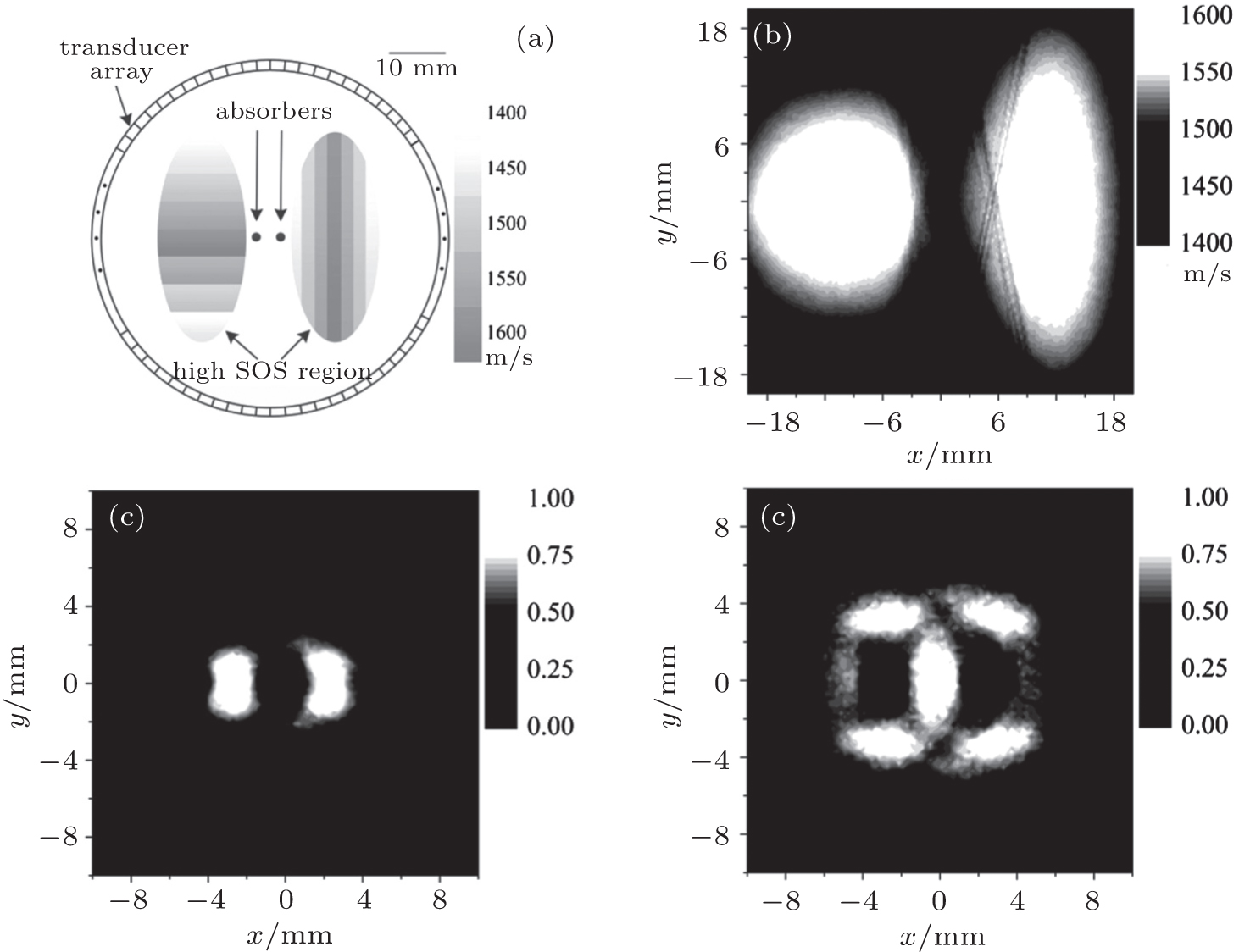 | Fig. 8. (a) Diagram of the simulation setup. The dark gray dots are optical absorbers and the light gray ellipses are the SOS variance region and the SOS distribution is shown by the color bar. (b) The SOS distribution estimated by US-CT. (c) The reconstructed PAT image by the CT-corrected DAS. (d) The reconstructed PAT image by DAS. |
In this study, we combine US-CT and PAT to obtain a high-quality PAT image of the acoustically inhomogeneous tissue with SOS variance. In the proposed method, the SOS distribution is recovered by an US-CT procedure. Using the recovered SOS information, a CT-corrected DAS method is employed to reconstruct the image from the PA signals. The simulation results validate that the proposed method can obtain a much better PAT image than the conventional DAS method when the SOS variance of the tissue is increased. In addition, we also find that the proposed method has a good performance even when the SOS variance reaches 14.2%. It is competent for imaging the soft tissue with inhomogeneous SOS distribution. Finally, an optimized fan angle is revealed, which ensures the quality of the PAT image and reduces the cost of the hardware. In the proposed method, US-CT and PA signal detection share the same US transducer array. The achievement of the proposed method does not need to add many extra hardware to the classical PAT system. Therefore, the proposed scheme could be easily integrated into a classical PAT system and improve PAT of the acoustically inhomogeneous tissue with SOS variance.
| 1 |
|
| 2 |
|
| 3 |
|
| 4 |
|
| 5 |
|
| 6 |
|
| 7 |
|
| 8 |
|
| 9 |
|
| 10 |
|
| 11 |
|
| 12 |
|
| 13 |
|
| 14 |
|
| 15 |
|
| 16 |
|
| 17 |
|
| 18 |
|
| 19 |
|
| 20 |
|
| 21 |
|
| 22 |
|
| 23 |
|
| 24 |
|
| 25 |
|
| 26 |
|
| 27 |
|
| 28 |
|
| 29 |
|
| 30 |
|
| 31 |
|
| 32 |
|
| 33 |
|
| 34 |
|
| 35 |
|
| 36 |
|
| 37 |
|