


A new collision avoidance model for pedestrian dynamics*
[Wang Qian-Linga) , Chen Yaob) , Dong Hai-Ronga)†  , Zhou Min
a) , Ning Bina) ]
, Zhou Min|
|


†Corresponding author. E-mail: hrdong@bjtu.edu.cn
Project supported by the National Natural Science Foundation of China (Grant Nos. 61233001 and 61322307) and the Fundamental Research Funds for Central Universities of China (Grant No. 2013JBZ007).
The pedestrians can only avoid collisions passively under the action of forces during simulations using the social force model, which may lead to unnatural behaviors. This paper proposes an optimization-based model for the avoidance of collisions, where the social repulsive force is removed in favor of a search for the quickest path to destination in the pedestrian’s vision field. In this way, the behaviors of pedestrians are governed by changing their desired walking direction and desired speed. By combining the critical factors of pedestrian movement, such as positions of the exit and obstacles and velocities of the neighbors, the choice of desired velocity has been rendered to a discrete optimization problem. Therefore, it is the self-driven force that leads pedestrians to a free path rather than the repulsive force, which means the pedestrians can actively avoid collisions. The new model is verified by comparing with the fundamental diagram and actual data. The simulation results of individual avoidance trajectories and crowd avoidance behaviors demonstrate the reasonability of the proposed model.
Nowadays, the gathering of people in public places, such as stations, stadiums, shopping halls, and so on is very common. This brings serious safety problems especially when emergency and critical situation occur. It may cause squeeze and stampede, even casualties. Therefore, it is important to understand the behaviors and dynamics of pedestrians and crowds in order to characterize their behaviors exactly during emergencies.
Researchers began to pay attention to this area nearly five decades ago.[1, 2] In the 1970s, Henderson presented the speed/velocity probability density distributions for different human crowds.[3] Fruin studied the factors that affect the planning and design of pedestrian spaces.[4] The initial work was mainly based on direct observations or photographs. However, they are not suitable for the prediction of the pedestrian flow in exceptional architectures or in evacuation situations.[5] Hence, all kinds of models have been proposed to simulate the flow of crowds and they are generally classified into macroscopic and microscopic models. For instance, the hydrodynamics models belong to macroscopic models which are the analogy of fluid and gas dynamics.[6– 8] Since the macroscopic models are described by the mean values of the characteristics of pedestrian crowds, they are more applicable when the crowds are large and individual differences are less important. Microscopic models include cellular automaton (CA) models, [9– 11] the pedestrian-following model, [12– 15] force-based models, [16– 18] etc. These models are very suitable for depicting the interaction behaviors between pedestrians.
In the CA model, the area is divided into cells of equal shape and the status is updated according to some rules at each time step, which makes it easy for computer simulations. A great deal of work has been done based on CA models. Zarita et al.[19] proposed a modified CA model to simulate an evacuation process in a classroom. They took into account the pedestrian’ s ability of selecting the exit route in their model. Li et al.[20] extended the CA model based on the floor field to study the pedestrian counterflow on a crosswalk. Lu et al.[21] also proposed an extended floor field CA model and used it to describe the walking behaviors of pedestrian groups. Their simulation results revealed that the presence of pedestrian group retards the emergence of lane formation and increases the instability of pedestrian flow. The pedestrian-following model was originally derived from the car-following model, which is the analogue of Newton’ s equation for each individual particle in a system of interacting classical particles.[22] In Ref. [21], the authors also introduced the leader-follower walking pattern, but Tang et al.[12, 13] carried out more in-depth research about the pedestrian’ s following characteristics. They proposed individual-following models for car, bicycle, and pedestrian. By applying the relationship between the micro and macro variables, they obtained a dynamic model for the heterogeneous traffic flow and derived some important results about the friction effects and honk effects.
The social force model[16] is another kind of prominent model for pedestrian dynamics. It can reproduce many self-organization phenomena observed in reality, such as lane formation, oscillation of passing direction at narrow passage, and the emergence of unstable roundabout traffic at intersections.[23] Based on this model, some researchers have made some improvements to study the pedestrian flow[24, 25] and evacuation problems.[26, 27] Other researchers mainly focused on the model itself and make some improvements to make it more realistic. Lakoba and his coworkers[28] proposed some algorithms considering the overlapping problem between pedestrians and the choice of the numerical values of parameters. Zarita et al.[29, 30] incorporated some decision-making and investigating capabilities and prediction factors in the social force model considering the intelligence of pedestrians. Nevertheless, the price of the precision by adding factors and modifying the formulas is a more sophisticated mathematical expression of the model.
Since most of the methods lack anticipation and prediction, the pedestrians’ behaviors may look unnatural and contain undesirable oscillations when they get too close.[31] Therefore, another aspect of modifying the social force model is to introduce the maneuver of avoiding collisions. Karamouzas et al.[31] presented a collision avoidance model based on collision prediction. In their model, the pedestrians scan the environment and detect future collisions, then they avoid collisions via an evasive force. Chraibi et al.[32] modeled the desired direction in force-based models which can be used in geometry characterized by the existence of corners. Zanlungo et al.[33] introduced a specification of the social force model in which pedestrians can explicitly predict the next collision in order to avoid it. They took the interaction force as a function of relative positions, velocities, and absolute velocity.
However, those modified models still belong to the force-based modeling framework. There are some problems with the force models that have been pointed out by Moussaï d et al.[34, 35] For instance, it is difficult to capture all the crowd behaviors in one model and some theoretical issues exist for the superposition of binary interactions. The reason is thought to be that the force-based models try to describe directly the observed movements of pedestrians rather than the internal cognitive processes that lead to the movements. In Ref. [34] they used some simple rules to generate the movement from the bottom to the top by describing the underlying cognitive processes used by the pedestrians. On the other hand, Tang et al.[14, 15] pointed out that most of the above models did not explicitly take into account the pedestrian’ s following behavior, so they cannot describe the pedestrian-following property. The phenomenon of “ following the crowd” in panic situations has been discovered by Helbing et al.[36] In normal situations, the environment and other pedestrian (neighbors) around a pedestrian also have some effects on his walking behaviors, among which the front pedestrians and associated factors of headway and relative velocity play important roles. Tang et al.[14, 15] proposed a new pedestrian-following model and applied it to aircraft boarding. Here, we also consider the neighbors’ effect and use a method similar to that in Ref. [34] to model the desired velocity including the value and the direction for the avoidance of collisions. By making some assumptions about the velocity relating to the gaps formed by the pedestrians around himself, it forms a discrete optimization problem. During the simulation, each pedestrian chooses his desired velocity by solving the optimization problem in each step. In this way, the social repulsive force in the social force model can be removed and the behaviors of pedestrians are governed by the pedestrians’ choices of desired walking direction and desired speed. Thus, the pedestrians can avoid collisions actively as real humans rather than particles or balls in the force-based models in which they can only passively move under the action of forces.
This paper is outlined as follows. Section 2 introduces the original social force model and proposes the optimization-based method to model the desired velocities for the collision avoidance of pedestrians. In Section 3, the simulation results show the model verification, individual avoidance trajectories, and crowd avoidance behaviors. An oscillation index which reflects the deviation of the actual velocities from the desired velocities is also defined. Section 4 ends with the conclusion and some possible future work.
Before modeling the desired velocity of a pedestrian, we first introduce the social force model which was first proposed by Helbing et al.[16, 36] In this model, the pedestrians are treated as self-driven particles and their behaviors are described by the physical and socio-psychological forces. The trajectories of each individual are determined by Newton’ s Second Law of motion. The fundamental dynamical equations are
where mi, xi, and vi represent the mass, position, and velocity of pedestrian i, respectively. The trajectory of pedestrian i usually has the shape of a polygon with edges 


where Ai, Bi, k, and κ are constants. rij = ri+ rj is the sum of pedestrian i and pedestrian j ’ s radii, and dij = || xi – xj|| is the distance between their centers of mass. nij is the normalized direction which points from pedestrian j to i and tij is the direction perpendicular to nij. 
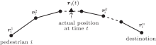
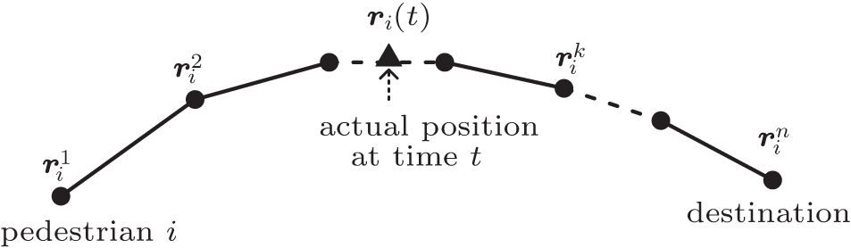 | Fig. 1. Illustration of pedestrian i’ s desired direction. |
In the social force model, it is assumed that the pedestrians want to reach a certain destination as comfortably as possible and make a trajectory without detours. The trajectory usually has the shape of a polygon, but the specific method to find the polygon is unclear. Besides, it shows some irrational simulation results using this model. In the following part, we propose an optimization-based method to calculate the desired direction by endowing some intelligent abilities to the pedestrians and making some assumptions about the desired speed.
As vision is the main source of information used by pedestrians to control their motion, [34] first we endow the visual ability to the particles which represent the pedestrians. Humans usually have an almost 180-degree forward-facing horizontal field of view, of which binocular vision covers only 120 degrees. The remaining peripheral 60 degrees have no binocular vision because of the lack of overlap in the images from either eye for those parts. As the binocular vision is just important for depth perception, we take 180 degrees as pedestrians’ visual field for simplicity, which means a pedestrian can see all the other people in front of him. More specifically, we assume that a pedestrian’ s vision field is related to his velocity direction, namely, the vision field of a pedestrian is 180 degrees with his velocity direction being the center line. Next, we can define the neighbors of a pedestrian i as
Ni(t) is the set of the neighbors pij at time t, and di represents the pedestrian i’ s neighbor scope which differs from person to person and is affected by individual’ s preference, environment, culture, and some other factors. The illustration of the neighbors of pedestrian i is shown in Fig. 2 (the obstacles can be treated equivalently with the pedestrians, for the obstacles can be seen as static pedestrians or the pedestrians can be seen as moving obstacles).
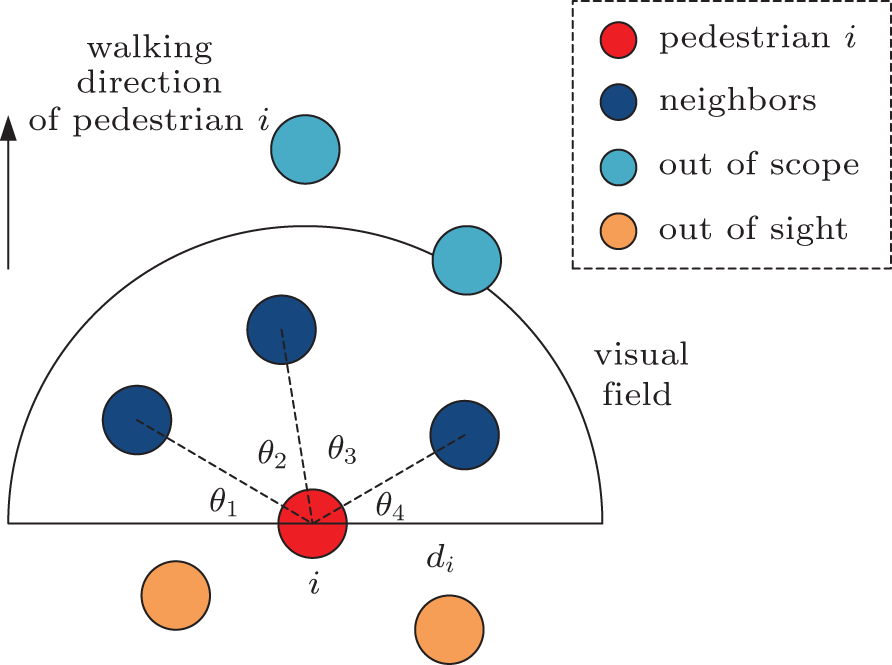 | Fig. 2. Illustration of the neighbors of pedestrian i. The pedestrians around pedestrian i can be classified into three types: the neighbors, the pedestrians who are out of neighbor scope, and those behind pedestrian i who are out of sight. |
It can be seen from the figure that the lines jointing pedestrian i and his neighbors and the horizontal line (the line which is perpendicular to pedestrian i’ s velocity direction) forms some angles represented by θ k(t). We can use these angles to represent the neighbors. Usually, if there are no other pedestrians on the horizontal line, the number of angles is one more than the number of neighbors.

Obviously, the number of θ k(t) is finite, so that pedestrian can choose one slot between two adjacent pedestrians to go through when his original walking direction is obstructed. Then it naturally leads to another question: which one should pedestrian i choose among these angles? We will explain this after making some assumptions about the velocity in the next part. To end this part, another kind of ability, the predictive ability, is endowed to pedestrians. It assumes a pedestrian can predict or perceive his neighbors’ positions and velocities, which can be used as part of the information for pedestrians to make decisions. It represents by the set Pi(t).

xij' (t) and vij' (t) are the position and velocity of pedestrian j perceived by pedestrian i, respectively.
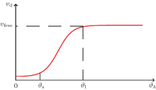
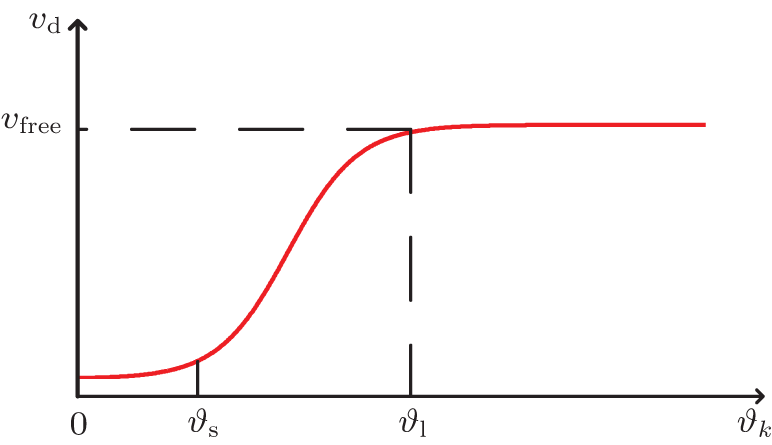
Previous studies have shown that the flow and velocity of the crowd are related to the bottleneck.[37, 38] Normally, the flow and velocity will increase as the bottleneck gets wide. If we treat the gap between two neighbors as a bottleneck, we can make an assumption that the desired velocity is related to the size of the gap. From another point of view, the velocity is related to the density of the crowd.[39] In general, the bigger density indicates the smaller pedestrian gaps. So we can assume, in microscopic aspect, the desired velocity has an exponential relationship with the angle which is similar to the Underwood model.[39] Moreover, when the gap is narrow, a pedestrian should go through it gingerly with a small velocity; while the gap is wide enough, he can walk through it freely. Hence, the desired velocity about the gap has the relation as shown in Fig. 3.
Here, vfree is the desired velocity when a pedestrian walks in an unobstructed place; ϑ s and ϑ l are the thresholds. When the gap is smaller than ϑ s, it means the gap is too narrow to go through for a pedestrian. A pedestrian can walk freely with velocity vfree when the gap is bigger than ϑ l. According to Fig. 3, we choose the s-curve function to approximately describe the relation (α and β are parameters)
where
reflects the size of the gap and dipk– 1(t) and dipk(t) are the distances from pedestrian i to the neighbors who form the gap k (if there is only one neighbor, we set the two distances equal to each other).
 | Fig. 3. Relation between desired velocity and the gap. |
In the above, we only consider the positions of the pedestrians to determine the velocities. However, the velocity of one pedestrian is not only related to the positions of other pedestrians but also to their velocities. A pedestrian should avoid collision with others considering the relative velocity. If 


Thus, the value of the desired velocity for pedestrian i at time t considering other pedestrians’ positions and velocities should be

From above analysis, it is clear that a pedestrian will change his desired direction and choose a gap formed by his neighbors to go through with the speed ||vdi(t)|| when he gets stuck. Then we determine the specific gap and direction that the pedestrian will choose.
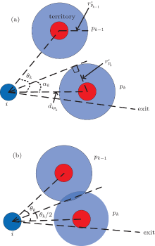
First is the specific direction which the pedestrian will go along. To begin with, the radius of pedestrian is redefined. In Ref. [40], the author proposed the proxemic behavior theory. It claimed that there are different spaces surrounding a person: intimate space, personal space, social space, and public space. In Ref. [41], the author proposed the “ fear to be touched principle” , namely, there is nothing man fears more than the touch of the unknown. Based on this principle, the pedestrian’ s radius is extended and a territory where the pedestrian does not want to be violated, and also others do not want to get close to, is given to each pedestrian. As shown in Fig. 4(a), 

When the environment is not crowed, as the pedestrian does not want to get too close to other pedestrians and also does not want to deviate too much from the direct path, he will choose the direction that is tangential to the territory of the neighbor who is closer to the direct path, namely, α k in Fig. 4(a).
where 
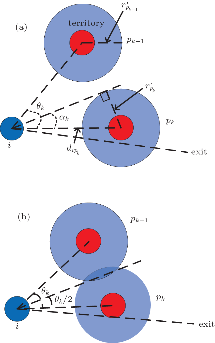 | Fig. 4. Illustration of the territory of a pedestrian and the desired direction. (a) The desired direction when the environment is not crowed. (b) The desired direction when the environment is crowded. |
When the environment is crowded, for example, pk and pk– 1’ s territories intersect each other, pedestrian i would go along the center line of θ k(t) (Fig. 4(b)). Therefore, the specific angle of the direction relative to neighbor pk after a pedestrian chooses θ k is

If the angle between line pedestrian i-neighbor pk and line pedestrian i-exit (the direct path) is ϕ k(t), then the angle of the desired direction relative to the direct path is

We next determine the specific gap (θ k(t)) the pedestrian will choose, namely, to determine the neighbor pk. Because the pedestrian wants to get to his destination as soon as possible, it is easy to assume that he will choose the direction in which the projection of his velocity to the direct path is the maximum (if more than one projections are equal, he would choose the one which deviates least from the direct path). That is,
This forms a discrete optimization problem. By solving this problem, we can find the specific gap.
To summarize, when a pedestrian gets stuck (that is there are some other people on his way to the destination and their velocities are smaller than his), he would change his desired direction and choose one of the gaps formed by his neighbors to go through. The directions along the center lines or tangent to the neighbors’ territories which are closer to the direct path are his choices. As we have made an assumption that the velocities about the gaps are different along each direction, the pedestrian would choose the direction in which he can get to the destination as soon as possible, that is the projection of the velocity to the direct path is the maximum. For the optimization problem is finite and discrete, we can always find the optimal solution. So the pedestrians can avoid collisions by changing their desired directions instead of the social repulsive force.
As mentioned above, the modeling of the desired speed and desired direction can replace the social repulsive force. It has incorporated the repulsive maneuver in the self-driven force rather than using the social repulsive force. When the environment is too crowded and the pedestrians have to touch each other, we use the “ body force” k(rij – dij) nij and “ sliding friction force” 
where

and

The function

||vdi(t)|| is determined by Eq. (8), ei(t) = (cos(η k(t)), sinη k(t)) is determined by Eq. (11), and the index k is determined by the optimization problem (12). Other symbols are the same as the social force model.[34] This model determines a pedestrian' s desired direction through local optimization (the information of neighbors of the pedestrian), and does not involve any global way-finding strategy, which may cause the oscillation of slot selection during the simulation. However, the modeling process can decrease the oscillation as much as possible. For a pedestrian, when his neighbors do not change, the slots change continuously over time, so does the optimization function (12); when new neighbors are added, the collision avoidance maneuver (7) can guarantee that the pedestrian does not choose the slot which will have the collision; the reducing of neighbors usually does not affect the slot selection. The simulation results also demonstrate that the pedestrians in the proposed model fluctuate less severely than those in the original social force model. Then we conduct the simulations using model (13) in the next part.
As a pedestrian accelerates or decelerates in response to the speed of his leaders or colliders within a range of up to 5.59 m and 3.863 m for low- and high-density cases, respectively, [43] we assume that the radius of the neighbor scope di for pedestrian i is approximated to be 4 m. For simplicity, we take this parameter to be the same for all pedestrians. As for the parameter ϑ s in Section 2.3, when the gap between two neighbors is smaller than one person’ s dimension, the person cannot go through it. Consequently, ϑ s = 0.5 if the person’ s radius is 0.25 m. If we take the territory of a person into account, when the gap between two neighbors is bigger than the person’ s dimension, he can go through it freely. As the personal distance of a person is about between 0.46 m and 0.76 m, [40] we take it as 0.8 m, the parameter ϑ l = 1.6. Then we choose α = 6 and β = 0.15. Actually, the values of these two parameters do not affect the simulation much. The position and velocity of pedestrian j predicted by pedestrian i are approximated by pedestrian j’ s real position and velocity. We set the time τ in Eq. (7) as 1 s.[44] The initial desired speeds of pedestrians are assumed to be Gaussian distributed with a mean value of 1.34 m/s and standard deviation 0.26 m/s.[17, 18] The other parameters of the modified model are as follows: k = 24000 kg/s2, κ = 1 kg/ms, m = 80 kg, and ri = 0.25 m.[28]
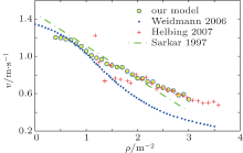
Since we have introduced new parameters and made modifications to the original social force model, we need to make sure that the new model can still be used to describe the behaviors of crowd. To verify a model, some researchers compare with the aggregate outcomes such as fundamental diagrams[18, 24] or well-known phenomena such as clogging, [17, 36] while other researchers use the maximum likelihood estimation method based on observed walking trajectories of pedestrians.[43, 45] Here we use the former method to verify the proposed model. First, we check the relationship between speed and density, which is known as the fundamental diagram. To measure the average speeds of crowds, we carry out some simulations in a corridor of 20× 2 m2 with periodic boundary conditions, and the density of pedestrians is varied from 0.4 to 3 p/m2. The density is calculated as the total number of pedestrians (N) over the total area of the corridor [(ρ = N/20× 2)]. For each density, we run the simulation ten times and each one runs for 50 s. The velocities of the pedestrians are recorded at every step size. The first 20 s of each simulation are discarded to ensure that all the pedestrians have reached their steady state. The velocity corresponding to that density is calculated by averaging over all pedestrians, iterations, and running times. The results are shown in Fig. 5 and compared with experimental data.[46, 47]
However, when the density is bigger than 1 p/m2, the speeds are higher than those in Ref. [48] and the explanations for the deviations between different fundamental diagrams include cultural and population difference, influence of psychological factors, the type of traffic, and so on.[49] In general, pedestrians in high density regions have slower speeds than those in low density regions.
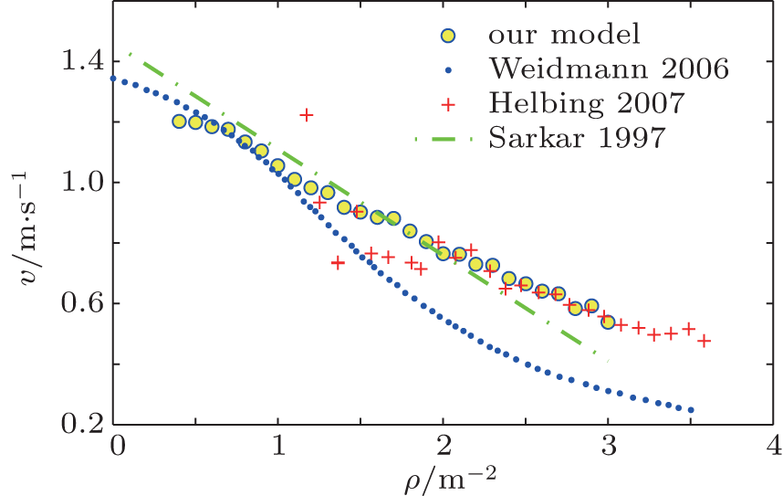 | Fig. 5. Fundamental diagrams for pedestrian movement and simulation results. |
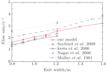
Another aspect is the pedestrian flow through bottlenecks. Some work has been done to analyze the flow rates through exits with different widths.[49– 53] Here, we use the relationship between flow rate and exit width as another benchmark to verify our modified model. To compare our simulation result to the previous work, we create a similar scenario to that in Ref. [50]. It is a room which is about 4 m wide with an exit on the middle of one side and 9 m long. For each run, 100 pedestrians evacuate from the room and the exits vary from 0.8 m to 1.6 m. The flow rate here is calculated as the total pedestrian number over the time interval [(100/tlast – tfirst)], where tfirst and tlast are the time when the first pedestrian and last pedestrian pass by the exit, respectively. Figure 6 shows the comparison result between our simulation and some experimental data. We can find that the flow rates predicted by our model lie within the range of flows reported by other researchers and show a linear dependence relation with exit width, which coheres with the result in Ref. [49].
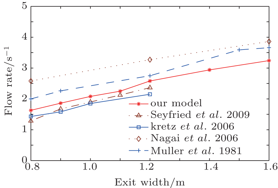 | Fig. 6. Flow rates with different exit width. |
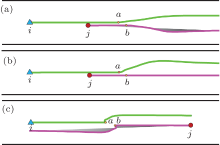
To make a better comparison, the simulations of avoiding collisions using the original social force model are first conducted. The walking trajectories are shown in Fig. 7. First, in Fig. 7(a), if we do not take the visual effect into account, each pedestrian would suffer the social forces from all the other people around him which means one will be affected by the behind pedestrians even though he cannot see them. So pedestrian j is repelled away by i at point b. Meanwhile, pedestrian i feels the repulsive force from j at point a. However in fact, the relationship between pedestrians does not necessarily show the “ action-reaction” or “ stimulus-response” law as in physics.[54] Most of the time the pedestrians in front pay little attention to what occurs behind them and are unlikely to notice anyone in the back.[55] Then, in Fig. 7(b), it considers the factor of visual angel. As it shows, the walking trajectory of pedestrian j is a straight line without being affected by pedestrian i. However, we observe the unrealistic behavior on pedestrian i. At point a, the closest position i can reach before he knocks into j, he stops suddenly and then changes his walking direction. This is also reflected in Fig. 7(c). Pedestrians i and j are bounced back a little due to the repulsive force at a and b, respectively, when they walk towards each other. Obviously, pedestrians do not walk like this in reality, they have beforehand preparations and plans when they see an obstacle.
After all, the reason causing those unrealities is that we treat pedestrians as particles or balls without thinking abilities. They can only passively avoid the collisions through repulsive forces. As a matter of fact, pedestrians have the thinking ability and all kinds of perception abilities. They can evade an obstacle or another pedestrian actively rather than wait to feel the repulsive force to take action.
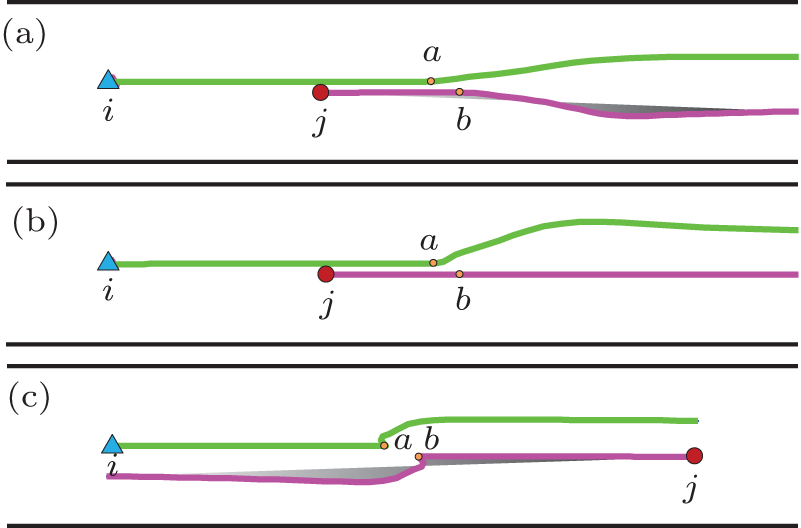 | Fig. 7. The walking trajectories of pedestrians simulated by the social force model. |
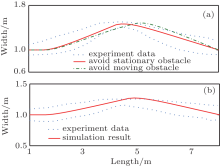
Then we simulate the avoiding collision behaviors of the single person using the modified model and compare the walking trajectory with the experiment data from Ref. [56].
In Ref. [56], the experimental corridor was 7.88 m long and 1.75 m wide and was equipped with tracking systems to record the trajectories of the subjects. In first scenario, a person was instructed to stand still in the middle of the corridor, while another one was asked to go from the left to the right and had to evade the standing person. We conducted simulations under the same conditions; the results are shown in Fig. 8(a). We can see the predicted path (red line) by our model lies within the standard deviation (blue dashed lines) of the real human paths. Besides, we also conduct the simulation of evading a moving pedestrian. That is, we let the person in the middle also walk towards the right side but with a smaller velocity. The path (green dashed line) is deviated to the right relative to the red line which is easy to understand because we need a longer process to avoid the moving person.
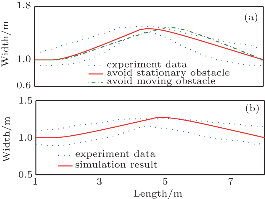 | Fig. 8. Simulation result compared with experiment data for avoiding collisions. |
In the second scenario (Fig. 8(b)), two pedestrians start from the opposite ends of the corridor and walk towards each other to exchange their places, therefore they have to evade each other. Again, we find that the predicted path by our model basically accords with the experiment data.
Comparing Fig. 7 and Fig. 8, it is easy to find that the trajectories in Fig. 8 are more realistic than those in Fig. 7.
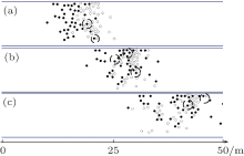
In this section, we simulate the collective behaviors which also involved the avoiding collision behaviors. We assume that there are 80 persons in a corridor with the size of 50 m long and 10 m wide. The initial positions of forty people (full circles) are in the left side of the corridor and the other forty (empty circles) are placed about ten meters ahead of them. The velocities of the latter forty persons are uniformly distributed with a mean value of 1.34 m/s, while the former forty persons are about 1 m/s slower than the latter ones. The two groups of persons interact in the middle of the corridor. We took some snapshots of simulation process. Figure 9 shows the original social force model and figure 10 shows the modified model. Comparing the two figures, we can see that a lot of full circles get stuck behind the empty circles in Fig. 9. This is because in the original social force model, the pedestrians cannot avoid the front people positively (but by forces). In Fig. 10, the full circles are in the interspaces of the empty circles as the pedestrians can change their desired directions and walk through the crowd.
In the above sections, we show the unrealistic simulating pedestrian behaviors of the original social force model in Figs. 7 and 9. The pedestrians would have a sudden stop or be bounced back when he gets close to another pedestrian. That is, his velocity would have a sudden change (oscillation) when his behavior becomes unrealistic. In this section, we analyze this in a more quantified way by defining the oscillation index of velocities.
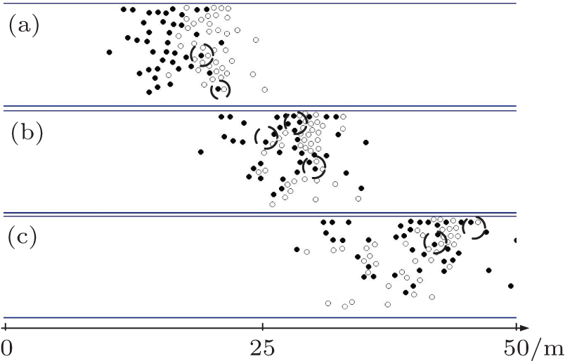 | Fig. 9. Snapshots of the simulation of pedestrians moving in the corridor using the original social force model. (a) t = 10 s, (b) t = 20 s, and (c) t = 30 s. |
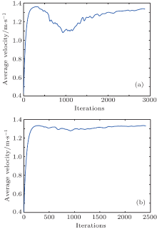
First, we calculate the average velocities of the crowds simulated using the original social force model and the modified model, separately, where the scenario is the same as that in Section 3.3. The results are shown in Fig. 11. We can see that the average velocity of the original model (Fig. 11(a)) fluctuates more severe than that of the modified model (Fig. 11(b)), especially during the iteration 500 and iteration 1500 when the two groups of pedestrians interact with each other. This means in the original social force model the velocities of pedestrians change more frequently, which also means the unrealistic behaviors occur more frequently than those in the modified model.
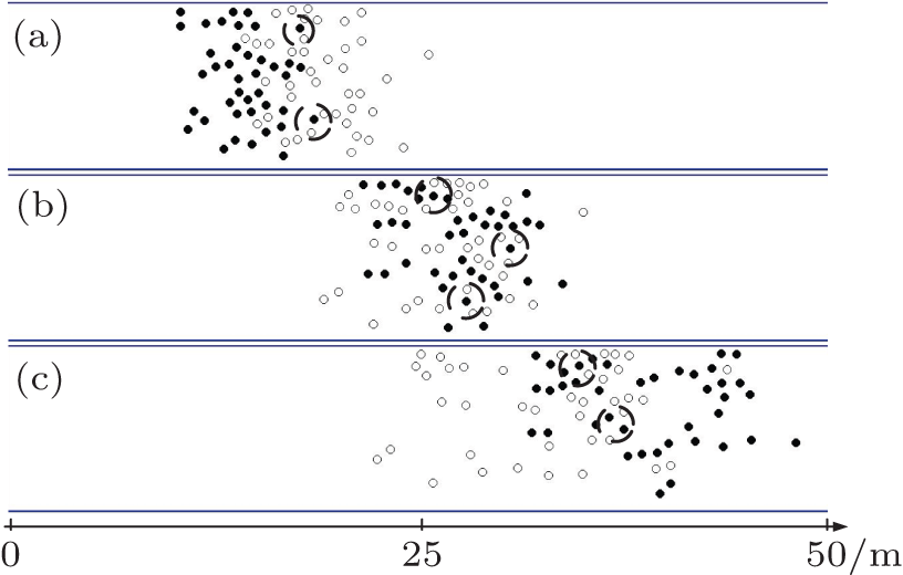 | Fig. 10. Snapshots of the simulation of pedestrians moving in the corridor using the modified social force model. (a) t = 10 s, (b) t = 20 s, and (c) t = 30 s. |
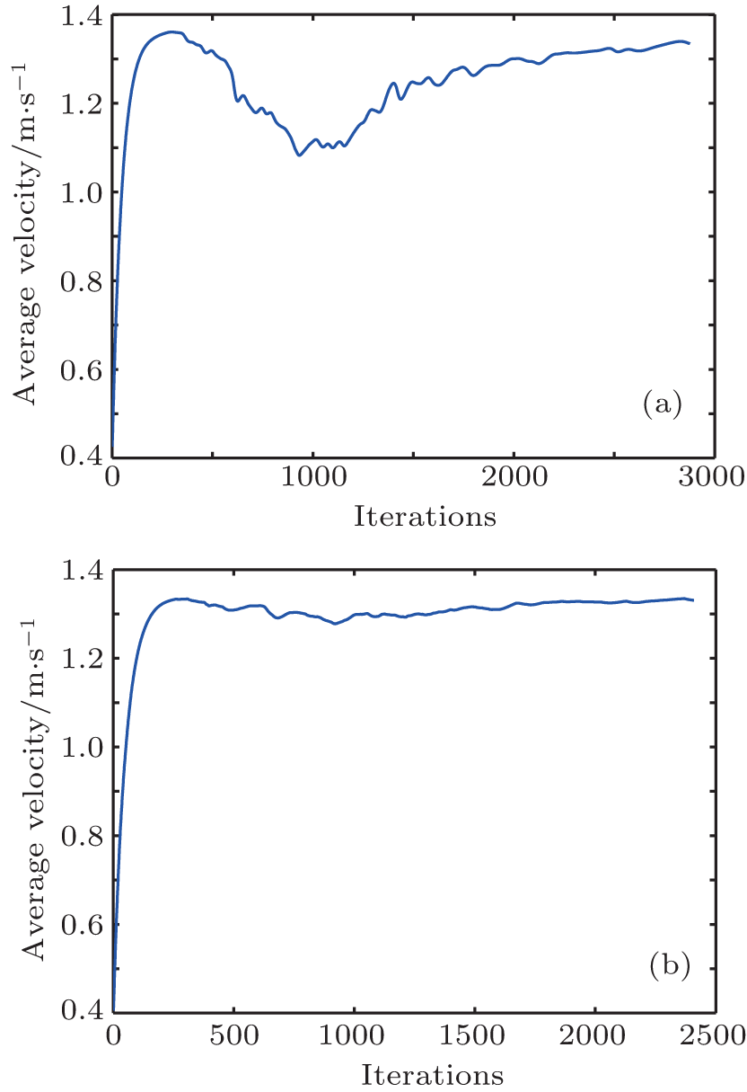 | Fig. 11. Average velocities of the crowds during the simulations using two kinds of models. (a) Simulation result using the original social force model. (b) Simulation result using the modified model. |
To describe the oscillations of the velocities in Fig. 11, we define an oscillation index in a similar way to that in Ref. [18]
where vi(t) and 
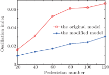
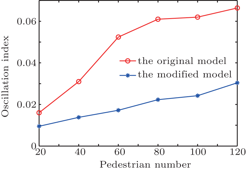 | Fig. 12. Oscillation indices of the original social force model and the modified model as functions of pedestrian number. The pedestrian number here is actually half of the total number, because there are two kinds of groups (the faster one and the slower one) in each run. |
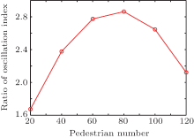
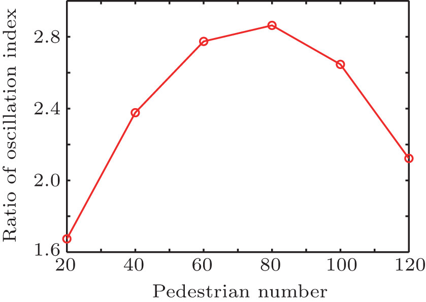 | Fig. 13. Ratio of the two kinds of oscillation indices (OI of original model/OI of the modified model). |
We can see both the oscillation indices of the two models increase as the pedestrian number (density) increases. Hence, this index reflects the chance of the interacting between pedestrians gets big as the density increases, which coheres with the reality. However, we can also find that the oscillation index of the original model is much greater than that of the modified model, which means that the velocities of the original model change more severe. Furthermore, the changing rates of the two kinds of oscillation indices are different when the pedestrian number varies. Then we calculate the ratio of the two kinds of oscillation index and make a quadratic fit (Fig. 13). The ratio first increases and then descends with the increase in the pedestrian number. This is because when the density is small, the pedestrians can walk freely and barely interact with each other; when the density is large, it is hard to go through the crowd for pedestrians in both models due to interactions. Thus, it has a better effect to use our model when the density of pedestrians is medium.
In summary, we have proposed a method to model the desired direction in the social force model. After making some assumptions to the pedestrians and velocities, we form an optimization problem. The pedestrian can change their desired direction to bypass the obstacles to avoid collisions by solving the optimization problem. We made the preliminary validation of the modified model by comparing with the fundamental diagrams and the experimental data. Then we simulate the avoiding behaviors for one single person and the crowd. The results show that the predicted paths of the modified model fit well with that of the real-world humans and the behaviors are more realistic. We also define an oscillation index to reflect the changing of velocities. The results show that the velocities of the original model have more severe fluctuations than those of the modified model.
Though the modified model can reproduce more realistic behaviors, we still need further validation and verification for modeling more complex behaviors and more complex scenarios. In the future work, the assumption about the velocities needs to be verified by control experiments. The parameters of the model should be calibrated more elaborately based on observed data. The trajectories between the simulated and real pedestrians will be compared to further support the advantage of the proposed model and understand the behaviors of pedestrians better.
| 1 |
|
| 2 |
|
| 3 |
|
| 4 |
|
| 5 |
|
| 6 |
|
| 7 |
|
| 8 |
|
| 9 |
|
| 10 |
|
| 11 |
|
| 12 |
|
| 13 |
|
| 14 |
|
| 15 |
|
| 16 |
|
| 17 |
|
| 18 |
|
| 19 |
|
| 20 |
|
| 21 |
|
| 22 |
|
| 23 |
|
| 24 |
|
| 25 |
|
| 26 |
|
| 27 |
|
| 28 |
|
| 29 |
|
| 30 |
|
| 31 |
|
| 32 |
|
| 33 |
|
| 34 |
|
| 35 |
|
| 36 |
|
| 37 |
|
| 38 |
|
| 39 |
|
| 40 |
|
| 41 |
|
| 42 |
|
| 43 |
|
| 44 |
|
| 45 |
|
| 46 |
|
| 47 |
|
| 48 |
|
| 49 |
|
| 50 |
|
| 51 |
|
| 52 |
|
| 53 |
|
| 54 |
|
| 55 |
|
| 56 |
|