


V–L decomposition of a novel full-waveform lidar system based on virtual instrument technique
[Xu Fan† , Wang Yuan-Qing‡]
, Wang Yuan-Qing‡]
|
|


†E-mail: alextsui918@gmail.com
‡Corresponding author. E-mail: yqwang@nju.edu.cn
*Project supported by the National Natural Science Foundation of China (Grant No. 608320036).
A novel three-dimensional (3D) imaging lidar system which is based on a virtual instrument technique is introduced in this paper. The main characteristics of the system include: the capability of modeling a 3D object in accordance with the actual one by connecting to a geographic information system (GIS), and building the scene for the lidar experiment including the simulation environment. The simulation environment consists of four parts: laser pulse, atmospheric transport, target interaction, and receiving unit. Besides, the system provides an interface for the on-site experiment. In order to process the full waveform, we adopt the combination of pulse accumulation and wavelet denoising for signal enhancement. We also propose an optimized algorithm for data decomposition: the V–L decomposition method, which combines Vondrak smoothing and laser-template based fitting. Compared with conventional Gaussian decomposition, the new method brings an improvement in both precision and resolution of data decomposition. After applying V–L decomposition to the lidar system, we present the 3D reconstructed model to demonstrate the decomposition method.
As an active remote sensing technique, lidar has been widely used and developed into many kinds of measurement mechanisms applied in different fields.[1, 2] For the focal plane array imaging lidar, as shown in Fig. 1 the modeling, simulation and analysis of full-waveform are considered as the most important research contents for 3D imaging.[3, 4] The production and improvement for experiment equipment undoubtedly requires repeated validation on the simulation models, especially penetrating into most of the crucial details. On the aspect of researches on modeling and simulation, many successful cases come into being. The Lincoln laboratory developed a 3D lidar system based on the OpenGL platform, which is to simulate the airborne 3D ladar test concealed under the foliage. Through the analysis of the results, the matching degree between the simulation and on-site trial is within 20%.[5] Berginc and Jouffroy conducted the simulation of the 3D ladar sensor including physics-based modeling of laser backscattering from complex rough targets, reflectance modeling of porous occluders, development of 3D scenes, and reconstruction algorithms for identification.[6] Graham developed a Matlab-based testing platform, which built a 3D visualization scene through loading different types of 3D model data. The purpose of the simulation was to thoroughly study the performance of foliage penetrating ladar in different flight paths.[7] Kim et al. established a Monte Carlo model of a laser penetrating into trees, in order to obtain the full-waveform of lidar. The model combined lidar systems with natural scenes, including the atmosphere, trees and terrain, and ultimately finished with 3D vegetation modeling and a study on reflection characteristics.[8] Jutzi and Stilla simulated the slopes of different gradients, from which the echo waveforms were obtained. Through measuring the correlation between the measured wave and the estimated one, the gradient of slope was determined.[9, 10]
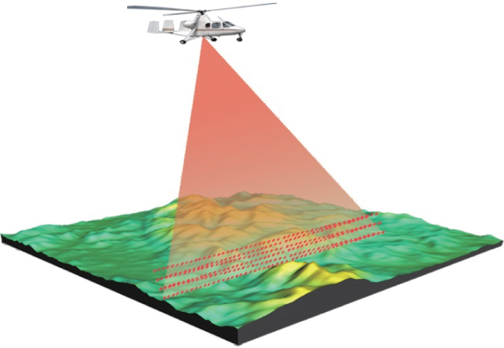 | Fig. 1. Diagram of airborne array laser radar. |
With the success of Quick Terrain Modeler, Terrasolid, Polyworks, and many other commercial softwares, the solutions for point cloud data processing and 3D imaging are becoming more and more mature.[11– 14] However, the processing and imaging tools are not seamlessly connected with laser imaging hardware systems. The point clouds uploaded by the receiver side of the lidar hardware system, must be preprocessed to fit the requirement for data form, storage format, and some other compatibility options. The redundant and onerous work counts against hardware and software integration of the whole laser systems, which increases the time cost, and reduces efficiency of processing and imaging.
Virtual instrument technology proposed by NI has been widely used in recent years. The virtual instrument is a computer-based hardware and software platform, which utilizes efficient software architecture to seamlessly integrate computer hardware devices with the new communication technology. The technology makes full use of the powerful computing performance of the computer to provide a software-based test and control solutions for data display, storage, and analysis. Generally speaking, virtual instrument technology greatly improves the flexibility and scalability, while saving the hardware costs and time costs. However, although virtual instrument technology has been extensively used in wireless communications, automatic control, and many other fields, it is rare to incorporate its advantages into the laser radar imaging, which is in urgent need of collaborative work of softwave and hardware. Abundant function libraries and subprograms, like 3D visualization, data acquisition, signal processing, field-programmable gate array (FPGA) development, I/O drivers, transmission control protocol (TCP) communications, etc., are integrated in a virtual instrument software development platform. Additionally, compatible interfaces for different development tools are available, and the novel graphical development language together with intuitionistic human– computer interaction are outstanding. It can be foreseen that the applications of virtual instrument technology in the laser radar system will certainly improve system integration and work efficiency.
In the present paper, we propose a systemic solution and an implementation for 3D imaging laser radar based on virtual instrument technology. The structural framework of our system is first provided, and then each component of it is mathematically modeled and analyzed. Specifically, a 3D scene for lidar that is built with geographic information system (GIS) data is designed. A simulation system setting platform, which is used to simulate the outdoor environments, is established. Also, a multi-channel data acquisition system, together with an upper monitor is designed and developed for site trial. The full-waveform data processing system, which consists of different algorithm modules, is systematically illustrated. Specially, we present an optimized algorithm for data decomposition, in which the Vondrak smoothing and laser– template-based fitting algorithm is adopted. Meanwhile, we give the evaluation criterion to demonstrate its superiority. Finally, the whole lidar system is presented and tested, according to which we make the analysis and draw some conclusions.
As mentioned before, the whole laser radar system is developed based on the virtual instrument, which consists of five main parts: 3D modeling, simulation environment modeling of the system, data acquisition system & upper monitor, full-waveform data processing, and 3D reconstruction. The overall structure is shown in Fig. 2. In the 3D scene modeling module, we aim at developing and utilizing the interface to 3D models, which makes the platform capable of loading 3D model files of different types, such as 3D terrain, 3D vegetation, and other surface features, and finally at building a 3D scene for laser radar trial. Simulation environment modeling of the system finishes the mathematical modeling of the environment in accordance with on-site trial, like the laser pulse model, atmospheric transport model, target interaction model, receiver model, etc. The pulse beams transmit in the environment, and eventually form a full-waveform with a certain signal-to-noise ratio (SNR). On the other hand, the full-waveform acquired from the on-site trial will be collected by the data acquisition system and then uploaded into the upper monitor on the computer side. The full-waveform data processing module is to complete the processing for a digital full-waveform (simulated or on-site), and then to decompose the intensity and depth data. Further, the decomposed information is utilized to build the 3D image of the target.
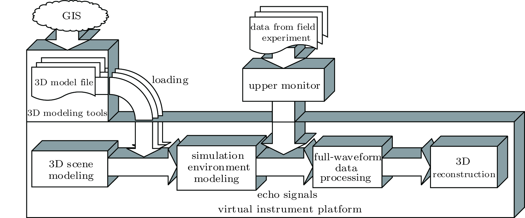 | Fig. 2. System structure of 3D laser radar system. |
Specifically, there are many researchers focusing on the optimization of decomposition for waveform radar to improve the system performance, which turns out to be effective. In terms of our radar system, the echo signals are sensed and amplified via an avalanche photodiodes (APDs) array (linear mode), and transmitted through a multi-channel data acquisition system up to the upper monitor. The cloud data obtained in the computer are digital waveform data with a certain SNR and sampling rate. In order to achieve effective decomposition of waveform and improve the resolution and precision, we propose a complete set of data processing programs, and design some optimized algorithms. For instance, we combine the pulse accumulation, wavelet de-noising with the Vondrak smoothing method to enhance and optimize waveforms. As a novel decomposition scheme, nonlinear fitting algorithm based on the laser template is designed in place of the Gaussian fitting. Accordingly, an appropriate evaluation criterion for goodness of fit is proposed. More details will be illustrated in the following section.
As described in Section 2, our system consists of five parts: 3D modeling, simulation environment modeling of lidar, data acquisition system & upper monitor, full-waveform data processing, and 3D reconstruction.
LabVIEW development platform provides interfaces for general 3D model files like VRML, STL, ASE, and many scene control methods, including background color, light source, perspective controller, automatic projection, display mode, and many other basic settings. Besides, setting options for texture, rotation, scale, translation are also available. Through selective and flexible use of these function controls, finally we can construct and render the desired scene. Modeling methods for 3D model files in the lidar system can be various and flexible. For instance, the terrain modeling can be finished with terrain plugin in 3dsmax, which can generate most of our required positions (different latitudes and longitudes) on earth by connecting the GIS. Trees and planes can be modeled in most 3D modeling tools like 3dsmax, AutoCAD, Solidworks. The above-mentioned 3D models are exemplified and shown in Fig. 3. Our target is to integrate different 3D models, configure appropriate setting options, and generate the desired scene for lidar simulation according to our actual requirements.
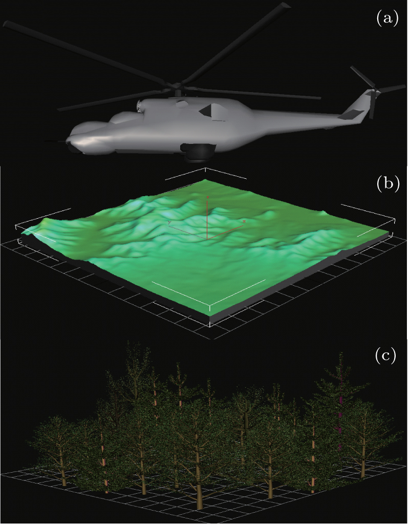 | Fig. 3. (a) 3D models of aircraft. It is designed to represent the airborne laser platform, which is located above the terrain and moves with the laser scanning. (b) 3D model of terrain. It is acquired from GIS system via a certain longitude and latitude, which contains geographic distribution data around the Earth. (c) 3D model of vegetation. It is designed to construct the forested areas representing the non-ground objects above the terrain. Appropriate location, height, branch parameters, density, and many other parameters for single tree need to be determined. |
Simulation environment modeling for the lidar system is so crucial that it is directly related to the proximity between the simulation and the site trial. In other words, the authenticity of the simulation environment models reflects the practicality of our system.
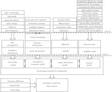
This subsection is devoted to building four models: the laser pulse model, atmospheric transport model, target interaction model, and the receiver model. Tomas[11] has made an overall mathematical model and also a detailed conclusion. Here, all of the above models are summarized as follows to illustrate the application in our system, and the entire structure of environment modeling is presented in Fig. 4.
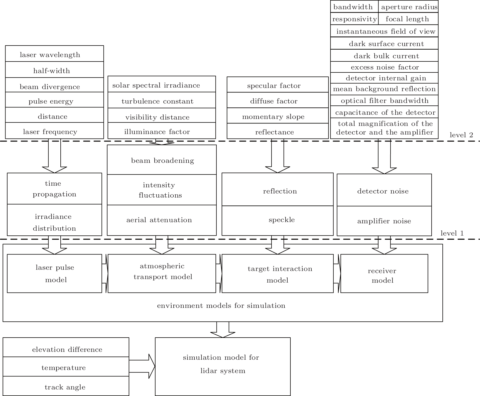 | Fig. 4. Structure of environment modeling for simulation. The input parameters for the module are classified as two levels. The 1st level input parameters are the most directly related to each model, while the 2nd level parameters are the more detailed explanations of 1st level parameters. To generate the final simulation model, some additional inputs, like elevation difference, temperature, and track angle are taken into account. |
(i) Laser pulse modelling is to describe the time propagation and irradiance distribution with the mathematical model. The former is described as[15, 16]

where T1/2 is the full width at half maximum, while the latter is

(ii) The target of atmospheric transport modelling is to describe the effects of beam broadening, intensity fluctuations, and aerial attenuation on the laser beam during the process of transmission.
The rule of beam broadening is

where 
The probability density function of the scintillation is
where 

The aerial attenuation results from the absorption and reflection effect by the particles in the air, which can be described as

where

The parameter q is a variable relating to visibility distance VM.
(iii) When the laser beam hits a diffuse surface of the target, the laser will be reflected into many directions, which results from effects of both diffuse and specular refection. Furthermore, the produced beams are independent and randomly phased, thus making dark and bright spots, which are called speckle cells, after they have interfered. The refection expression is
where A and B are correlation factors between diffuse and specular refection.
The speckle directly affects the waveform, which is different from the conventional additive noise, but a kind of multiplicative one. The probability density function of speckle values follows:

where M= Drec/Dsp, with Dsp = λ /ϕ , and Drec being the radius of optical input at the receiver.
(iv) Receiver model is modelled according to the noise equivalent power (NEP) from the detector and the amplifier, which can be expressed as


Since both of the expressions are representations of additive noise, the total NEP can be described as

The main parameters involved are explained as follows: ec is the electronic charge; B is the bandwidth; Ids is the dark surface current; Idb is the dark bulk current; Ib is the background illumination current; Is is the signal current; M is the detector internal gain; F is the excess noise factor; ℜ is the responsivity; k is the Boltzmann’ s constant; T is the temperature in degrees Kelvin; N is the noise factor for the electronics; RL is the load resistor.
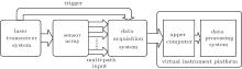
In order to make our system available for site trial, a simple prototype of the lidar system is designed. As shown in Fig. 5, the system consists of four main parts: a laser transceiver system, a sensor array, a data acquisition system, and a data upper-controlling and processing system.
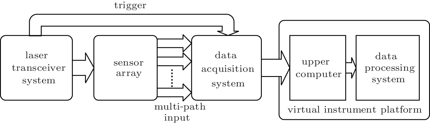 | Fig. 5. Diagram of our lidar system for site trial. |
The working principle can be described as follows. The receiver of the laser transceiver system emits a laser pulse at a constant frequency, while a sample of it is extracted to trigger and drive the data acquisition system after having been converted into an electrical signal. The echo signals are collected on the receiver side, and input into the sensor array. The output signals are analog electrical signals with a certain gain, and they are input into multi-channels of the data acquisition system. Multi-ADCs are controlled by an FPGA chip to work, simultaneously, after the trigger signal has come. The sampled data of multi-channels are aligned with a high accuracy, and transmitted into SSD. The upper monitor on the PC side can acquire data from SSD and convert them into decimal data, and then construct the full-waveform graph with data stored.
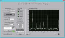
In the prototype system, a 532-nm laser is used, with an output frequency of 10 kHz. The sensor array we adopt is composed of four-unit APDs, each of which works in linear mode and generates an output of an electrical signal with a certain gain and with a certain noise suppression. The data acquisition system provides four interfaces for data input, one interface for the trigger signal input, and one interface for a high-frequency signal input as the sampling rate control. The highest sampling the system can reach is up to 1 Gs· ps. The data upper-controlling and processing system is located on the PC side with an Ethernet cable connected to a data acquisition system, which is developed based on the virtual instrument technology. The upper monitor and full-waveform display in the site trial is shown in Fig. 6. Since the frequency of the laser emitting is 10 kHz, echo signals appear periodically. When the object with special geometric characteristics is projected, multiple individuals return and overlap within the current period.
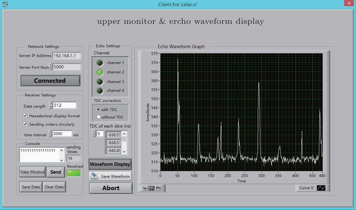 | Fig. 6. Software interface of the upper monitor over the Ethernet and the full waveform display. It is developed based on LabVIEW. The main setting parameters include an IP address and port number of server, data length, data format, sending mode, and time interval, etc. |
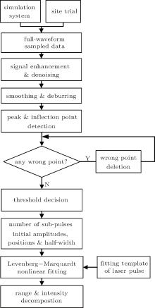
Full-waveform data processing system consists of three function modules, namely signal enhancement & de-noising, smoothing & deburring, and fitting & decomposition. The flow chart of full waveform data processing is shown in Fig. 7.
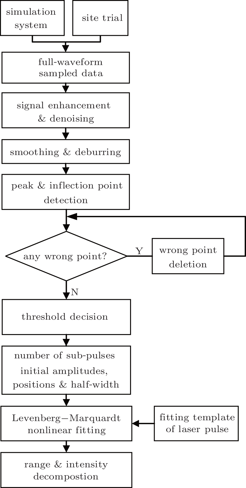 | Fig. 7. Flow chart of full waveform data processing. |
3.4.1. Signal enhancement & de-noising
As mentioned above, noise sources in the lidar system mainly come from atmospheric effects, target interaction, and receiver internal influence, which can be divided into two kinds, namely Gaussian noise and speckle noise. There are various effective methods for Gaussian noise; for instance, the wavelet denoising method has good time– frequency characteristics, and wavelet basis selection is flexible.[17, 18] Besides, wavelet denoising can deal with the edges, burr, and some other details of signals, to some extent. However, there is barely an effective processing method on speckle noise, which has been a bottleneck in the application of 3D imaging of the laser radar system. Owing to the multiplicative characteristic of speckle noise, a homomorphic filtering method is first considered. The principle is as follows: a noisy signal is first imposed on logarithmic transformation, thus converting the multiplicative noise into the additive; then frequency domain filtering is utilized to eliminate the ineffective part in the valid signal; finally the output signal is converted back to the original linear region by exponential transformation. The biggest problem of this method used in our system is that it requires a high performance in additive noise preprocessing, which is hardly realized in remote experiments and the low SNR condition.
Another method for dealing with a non-stationary random signal is the independent component correlation algorithm (ICA) method. Blanco et al.[19] applied it to speckle signals, and proposed a speckle ICA (SICA) method which takes into account the multiplicative model, and finally it is proved to be clearly improved on the basis of a standard ICA method for the speckle mixture condition. The limitation of this method is that it has a requirement for the number of noisy signal samples, and also has a higher algorithmic complexity.
Pulse accumulation has been widely used as an effective method for a non-stationary random signal in a radar system. Especially, on condition that the echo signals are weak and even when they are submerged in noise, this method is effective for improving SNR, to extract useful signals. Actually, pulse accumulation has good performances in noise suppression for both linear Gaussian noise and also speckle noise. Assuming S to be a useful signal, and N a random noise, the noisy signal within a cycle can be expressed as

After noisy signals in M cycles are added up, then
Then the SNR is
Since noises within different cycles are statistically independent of each other, namely

Thus
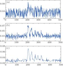
The above equation means that the effect of speckle noise, which is involved in the envelope of a useful signal, will become almost M times as great as the original effect after pulse accumulation. To sum up, we adopt pulse accumulation as an approach to signal enhancement and denoise preprocessing. Owing to the fact that the number of samples for accumulation is limited by the pulse frequency and the platform speed, the wavelet filter is utilized for further denoising. However, there is something more crucial that the improvement of SNR and the integrity of details of the waveform should be taken into account, simultaneously. On the basis of the principle, an appropriate wavelet base, filter length, and decomposition level are selected. The processing results of the above-mentioned de-noising methods in our system are shown in Fig. 8, from which we can demonstrate their efficiency quantitatively.
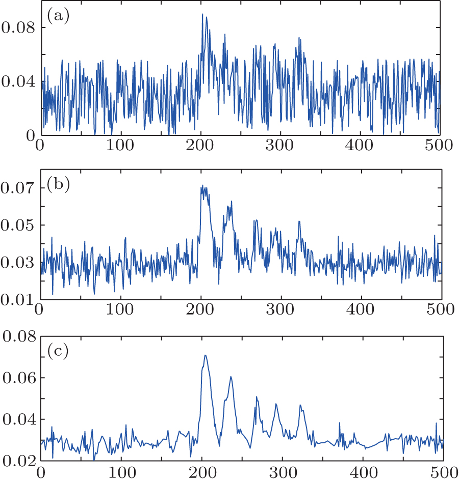 | Fig. 8. Diagram of waveforms after enhancement and de-noising. (a) The original echo waveform presents an SNR of poor quality, which is about − 5.95 dB; (b) after accumulation within eight cycles, the SNR is improved by about eight times, larger than before, namely 3.20 dB; (c) the result after wavelet filtering, which is significantly enhanced without missing the details of the waveform, the SNR of which is 9.38 dB. |
3.4.2. Smoothing
The purpose of the smoothing module is to deal with the detail problems of noisy signals, like local noise, burr, random fluctuation, etc. In this context, optimized signals are obtained, which are smoother and of higher SNR. There are some common smoothing methods, like polynomial smoothing, moving average, Gaussian smoothing, Vondrak smoothing, etc.
As mentioned above, one important principle for the noisy signal processing is to implement on the premise of ensuring the integrity of the wanted signal. To select an optimal approach as the smoothing module for our lidar system, various smoothing methods are compared. The Vondrak data smoothing method is proposed by an astronomer from Czech named Vondrak.[20] This smoothing method works well on condition that both the change regulation of observation data and functional form for fitting are unknown. The basic criterion of this method is

where

with x(ti) being the value to be smoothed. Here we define a parameter ε named the smoothing factor as the degree of smoothing, then ε = 1/λ 2, which means that the degree of smoothing increases as ε decreases. Figure 9 shows the effect of Vondrak smoothing on the echo data. As shown in the figure, the original data have many burrs. To smooth the waveform, we utilize the Vondrak smoothing methods of three values of smoothing factor ε = 100, 10, 1 (marked with a dashed line, dotted– dash line, and dotted line respectively). The results show that the smoothing result under ε = 100 remains good integrity while burrs are eliminated effectively.
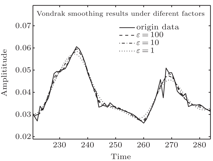 | Fig. 9. Vondrak smoothing results under different factors. Original data are marked with a solid line, which is smoothed with the three smoothing factor ε = 100, 10, 1 (marked with a dashed line, dotted– dash line, dotted line respectively). |
3.4.3. Fitting & decomposition
In order to identify the component of the full-waveform, the fitting & decomposition method is utilized to acquire the parameters like amplitude, position, and half-width of the different component. One effective and highly precise approach to full-waveform lidar decomposition is one nonlinear fitting method based on Levenberg– Marquardt (LM), which combines the local convergence characteristics of the Gauss– Newton iterative algorithm, also with global characteristics of the gradient descent, thus having faster iteration and higher accuracy. Specifically, Hofton et al. proposed one composition method, which combines the nonnegative least-squares method (LSM), and the LM method. The implementation procedure is described as follows.[21]
i) Corner detection is first used to determine the number of sub-wave components for the smoothed waveform.
ii) A pair of odd and even order corner points is used to determine the position and half-width of each Gaussian component. Then the initial amplitude estimates are obtained by using a nonnegative least-squares method (LSM).
iii) Different groups of parameters corresponding to different components are flagged and ranked, to select the useful components and reject the useless ones.
iv) To obtain much more precious decomposition results, the Levenburg– Marquardt method is utilized to optimize the former result. The input parameters are the initial parameter estimates, which includes amplitude, position, and half-width. The iterative formula is

where J(w) is the Jacobi matrix, u is the scale coefficient, r(w) is the residual vector, and Δ w is the iterative step.
However, most of the decomposition methods still regard the component of the full-waveform as the Gaussian form. This means that the full-waveform is expressed as

Actually, the time propagation of a typical laser pulse is described as

where τ = T1/2/3.5, with T1/2 representing the full width at half maximum. So there is obvious deviation because of using the Gaussian component fitting method. To eliminate the deviation, the fitting template needs to be amended according to Eq. (18). Then the new expression of a full-waveform is
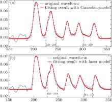
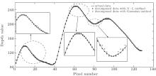
The fitting results with both the Gaussian model and laser model are shown in Fig. 10. In order to compare and evaluate the quality of fitting, we propose a criterion called the coefficient of determination (or goodness of fit): a greater coefficient of determination means a better fitting performance of the observed data and a more accurate result of decomposition. The coefficient of determination is defined as

where TSS means the total square sum of the observed data, expressed as 

where 
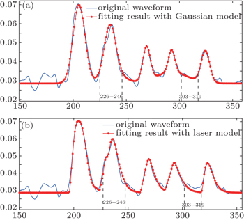 | Fig. 10. Fitting results based on (a) Gaussian template and (b) laser template on simulated echo waveform. Two specific ranges are marked in the figure, within which a comparison of goodness of fit between them is obvious. |
In Fig. 10(a), the value of R2 is 0.9934, while it is 0.9935 in Fig. 10(b). It seems that there is little difference in fitting performance between both of the fitting methods. Actually, it is inappropriate to calculate R2 directly through Eq. (22). Within the time range from 226 to 246, we find that the fitting result with the laser model is much better than with the Gaussian fitting, just under the same condition with other ranges around the pulse peaks. Contrarily, fitting with the Gaussian model performs better within those ranges around the tail (end) of the pulse, for instance, the ranges between 303 to 319 shown in Fig. 10. The reason is that the pulse tails are distorted more under the effect of certain intensity noise than the pulse peaks. Therefore, the criterion needs to be amended as follows:

In Eq. (23), we introduce a function W, which consists of a plurality of rectangular window functions, that is

where K is the number of rectangular window functions; RM j (n − nj) means the j-th rectangular window function, of which the width is M j, and the initial position is nj. Conventionally, RM (n) is defined as

Then the crucial point is how to determine the parameters K, M j, and nj. Here, we propose one method and its steps are as follows.
Step 1 Initialize parameters: K = N, i = 1, j = 1.
Step 2 Calculate the starting frequency and cutoff frequency of the specified threshold (e.g. 3 dB) of whole sub-pulses.
Step 3 Let 
Step 4 If 
Step 5 If 
As can be seen from the above, the updated method is essentially an approach to points’ selection and evaluation. With the new evaluation criteria, R̃ 2 can be obtained from Fig. 10, which is 0.9984 in Fig. 10(a) and 0.9988 in Fig. 10(b). It shows that there is a maximum deviation of two points in the decomposition result after Gaussian fitting, which means 0.3-m deviation when the sampling rate is 1 Gs· ps. Compared with the Gaussian model, the fitting result with the laser model has better goodness of fit and thus higher accuracy.
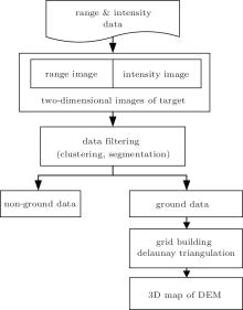
In this section, we are to use the depth and intensity information from the data processing module to generate a digital elevation model (DEM) of the terrain. The implementation process is shown in Fig. 11. Two-dimensional (2D) images, including both a range image and an intensity image, are produced from the decomposition data. Then data filtering is utilized to finish the clustering, segmentation on point cloud, which is classified as ground data and non-ground data. Data filtering algorithms for lidar have been refined in recent years. The basic principles of different algorithms are unified, i.e., a particular screening method is selected to eliminate the non-ground point and wrong point from the point cloud according to the difference in elevation information among different types. Specifically, a typical filtering algorithm based on triangular irregular networks is proposed by Axelsson.[22] The basic principle of the algorithm is described as follows. A sparse TIN is created from seed points, which are selected from those points with relatively low elevations within a sufficiently large area. Through an iterative method, the TIN network is constantly densified. The rule for densification is that the points from a new triangle mesh are added into the network once it satisfies the requirements for threshold constraint. The algorithm handles the surface with discontinuities in dense city areas. The commercial software TerraSolid adopts the algorithm as its filtering approach.
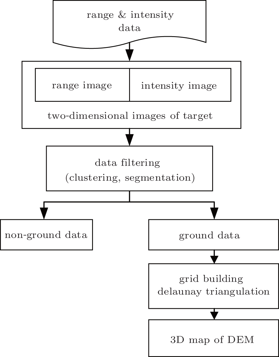 | Fig. 11. Flow chart of 3D reconstruction to build the DEM for Terrain object. |
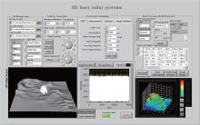
In this section, we present a 3D imaging laser system based on virtual instrument technology. We locate our laser experiment in the Taihang Moutains in China (Latitude: 38° 6′ N; Longitude: 114° 6′ E). According to the actual needs of our tests, the airborne laser is operated 1 km above ground level, acquiring 600-m swath wide data. Firstly, we obtain the digital Terrain data by connecting to a GIS, with which we produce a 3D model file with compatible format. Meanwhile, the 3D models of aircraft and vegetation are designed, which combines together with the Terrain model to be loaded into our laser test platform as shown in Fig. 12. Eventually, the laser test scene is built so that the digital surface model (DSM) is generated as shown in the lower left corner of Fig. 12. Our system will digitally record the full waveforms via an APD array and a data acquisition system, which are transmitted up to our platform by the upper monitor. The APD array consists of 64 photosensors, each of which works in the linear mode. The data acquisition system has 64 channels for waveforms input into 64 ADCs with a sampling rate of 1 Gs· ps, which works in parallel under the control of a single FPGA. Additionally, the time-to-digital converter (TDC) technology is introduced to improve the precision of the delay time, which is up to ps level. In order to avoid redundant data sampling and storage without leaving out useful points, we assume the elevation difference is 300 m. More detailed parameters of our laser radar system are shown in Table 1.
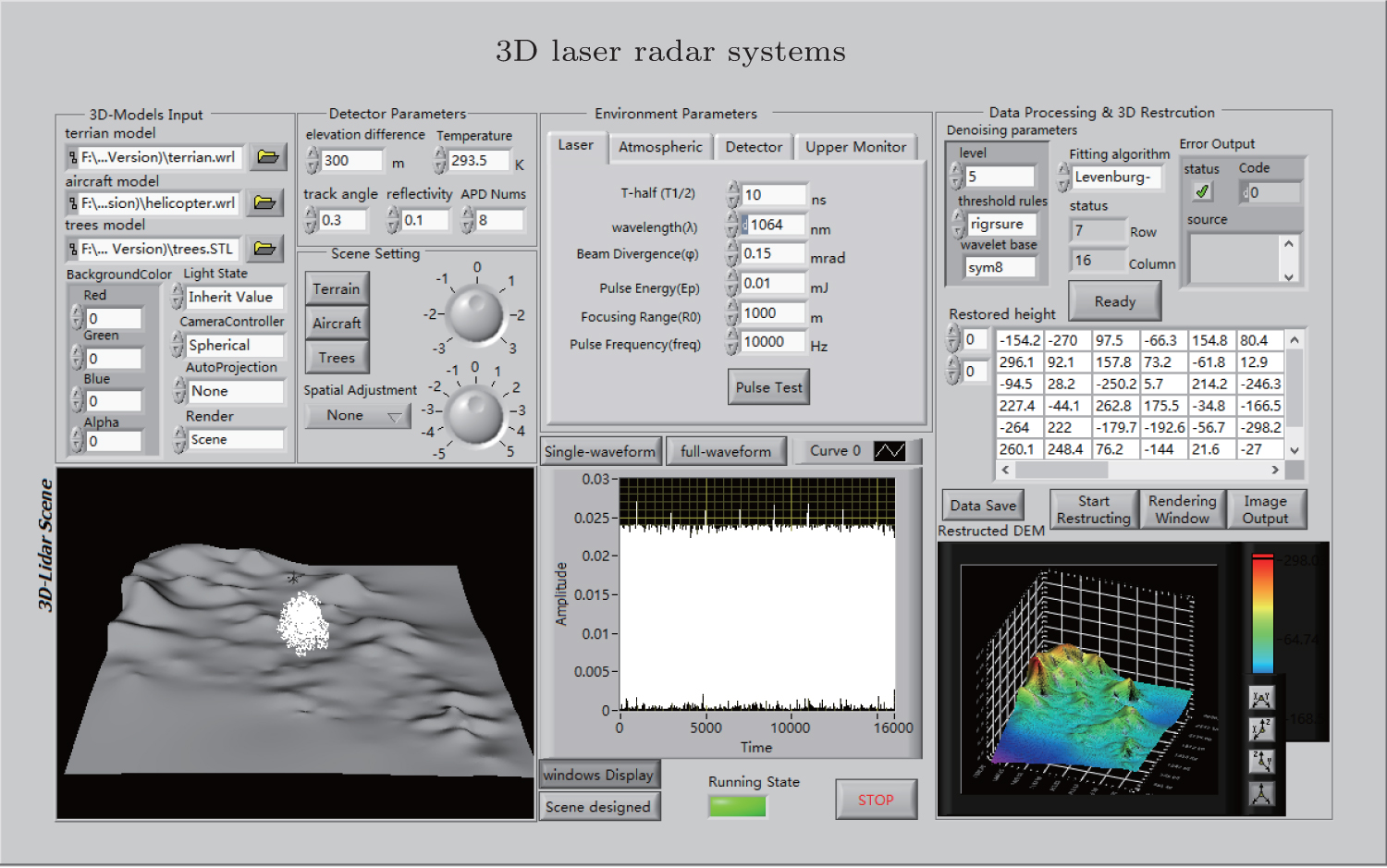 | Fig. 12. Software platform of 3D imaging laser radar system based on virtual instrument technology. Main modules are scene building, simulation modeling, upper monitor, data processing, and 3D reconstruction. |
| Table 1. Parameters of laser radar system. |
After obtaining a digitized full waveform, it is essential to perform the data processing. As illustrated before, after data enhancement and denoising, we utilize Vondrak fitting and the laser template-based decomposition method, which is called the V– L method here for simplicity. In order to judge the effect on data decomposition by the V– L method, we make a comparison with a conventional approach, which utilizes moving average fitting and the Gaussian decomposition method, which is shown in Fig. 13. In general, the average relative error brought by the V– L method is visibly lower than that by the Gaussian one, in which the former is 0.0075 when the latter is 0.0016. Therefore, it means that the precision of the V– L decomposition method is higher than that of the Gaussian one. On the other hand, those adjacent pixels that have little difference between each other (generally appear in areas with low gradient), are hardly to be distinguished between the two methods when the difference is beyond both of the resolution capabilities. Nevertheless, the number of indistinguishable points from the V– L decomposition is far less than that from the Gaussian one. That means that the V– L decomposition method also has a merit over the Gaussian method in high resolution.
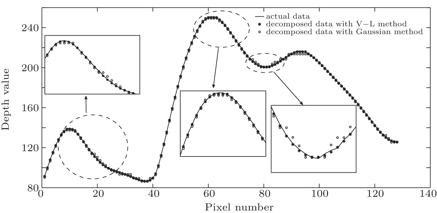 | Fig. 13. Comparison between V– L and Gaussian decomposition. We select 128 pixels from the target, which are used to implement decomposition. The results by the V– L method (represented by an asterisk), the results by the Gaussian method (represented by a circle) and the actual depth information (represented by a solid line) are all plotted. The dashed boxes shown in the figure are the enlarged views of three particular areas. |
The 2D range image is easily generated after the data cloud is decomposed. It can be found out that there are three types of points, namely the points of the ground surface, the points of the vegetation, and unknown points. The unknown points mainly result from the sudden change of elevation between adjacent points and inevitable error from data processing.
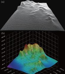
Then we need to execute the operation of filtering to finish classification and segmentation on the data cloud, which is to eliminate the unknown points and non-ground points and extract out the points of the ground surface. After the Delaunay triangular mesh is established, a TIN model of the digital elevation model is then generated as shown in Fig. 14(a). Subsequently, the interpolation and smoothing methods are adopted, which eventually finish and reconstruct the three-dimensional (3D) display of the digital elevation model as shown in Fig. 14(b).
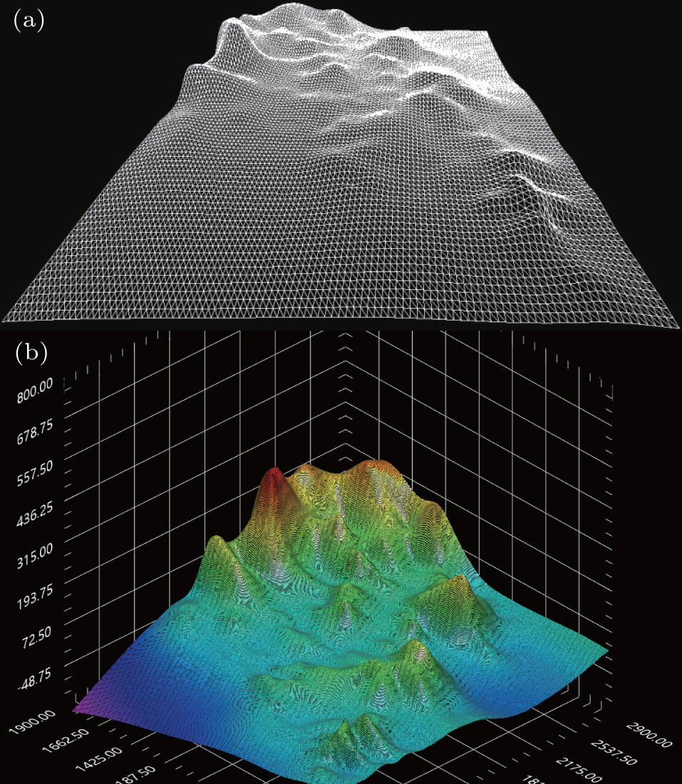 | Fig. 14. (a) TIN display for point cloud of Terrain object. (b) 3D display of reconstructed DEM. |
In this paper, we present a 3D imaging laser radar system based on virtual instrument technology. The system provides two functional approaches. One of the two approaches is that the system is capable of overall modeling and simulation for laser radar experiments in accordance with testing parameters, which includes modelling of 3D models, atmospheric environment, receiver, etc. The simulated full waveforms are processed through the data processing module, after which clustering, and segmentation are used to filter out the non-ground points and wrong points, and eventually the digital elevation model (DEM) of the Terrain is reconstructed. The other approach is provided for an on-site trial. After simulation, the appropriate detection altitude, the number of APDs and data processing methods are selected. We utilize a multi-sensor APD array to convert the collected optical waveforms into the electrical signal. The output is transmitted into the data acquisition system to produce the digitized full waveform data. Real time communication can be implemented to upload the digitized data to the computer via a serial port or Ethernet port connected to a data acquisition system, which benefits from virtual instrument technology. The subsequent data processing is executed with selected methods. The key attributes of the whole system can be summarized from two aspects as follows.
(i) The virtual instrument technology is introduced into the laser radar system, thus making a breakthrough in hardware and software integration and higher time efficiency. Meanwhile, 3D interfaces based on the virtual instrument platform are used to obtain Terrain data by connecting to GIS, bringing more intuitionistic 3D rendering.
(ii) In algorithm, we propose the V– L algorithm, which combines Vondrak smoothing and the laser-template-based fitting method, under which the evaluation method is designed. The results show that the V– L algorithm can effectively improve the resolution and precision of decomposed data.
Still, more work remains to be done. Firstly, the number of pixels needs to be increased. With urgent need for high resolution images, large-scale integrated APDs have been produced and used.[23] To make a breakthrough, we should make great efforts to overcome the difficulty. Secondly, our system is restricted by noise. Although the V– L algorithm improves precision and resolution of the decomposed results to some extent, it largely depends on the performance of the signal enhancement and denoising, especially under the condition of the remote detection. As to the realistic effect by a terrible noise environment, especially the speckle, an effective de-noising algorithm will greatly improve the range of the experiment. Finally, more functions of the system remain to be extended. The target of our system is to restore the 3D digital terrain map, while the practical application of lidar also pays much attention to the surface features. For instance, Reitberger et al.[24] proposed a novel segmentation approach for single trees based on full waveform lidar data. Compared with conventional watershed-based segmentation, the combination of the stem detection method and normalized cut segmentation brings better segmentation results. As for our system, it requires more detailed modeling for vegetation, to build a diverse vegetation database. In such a case, the 3D segmentation approach for single trees can be introduced. This definitely provides a new direction for further study.
| 1 |
|
| 2 |
|
| 3 |
|
| 4 |
|
| 5 |
|
| 6 |
|
| 7 |
|
| 8 |
|
| 9 |
|
| 10 |
|
| 11 |
|
| 12 |
|
| 13 |
|
| 14 |
|
| 15 |
|
| 16 |
|
| 17 |
|
| 18 |
|
| 19 |
|
| 20 |
|
| 21 |
|
| 22 |
|
| 23 |
|
| 24 |
|