Inter-particle interactions in many-body systems play a key role in determining the fundamental properties of the systems. In ultracold atomic gases, neutral atoms interact through the van der Waals force, which can be described by a contact potential characterized by a single s-wave scattering length. Such a simplification results in great success in cold atomic physics.^[1] For atoms possessing large magnetic moments, the long-range and anisotropic dipole–dipole interaction (DDI) may become comparable to the contact one, which leads to the dipolar quantum gases.^[2] So far, the experimentally realized dipolar systems include the ultracold gases of chromium,^[3] dysprosium,^[4,5] and erbium^[6] atoms. It is also possible to realize dipolar quantum gases with ultracold polar molecules.^[7–13] Compared to the short-range and isotropic contact interactions, DDI interaction gives rise to many remarkable phenomena, such as spontaneous demagnetization,^[14] d-wave collapse,^[15] droplet formation,^[16] and Fermi surface deformation.^[17]

Recently, a new quantum simulation platform based on atoms or molecules with electric quadrupole–quadrupole interaction (QQI) was theoretically proposed.^[18–24] The quantum phases of quadrupolar Fermi gases in a two-dimensional (2D) optical lattice^[18] and in two coupled one-dimensional (1D) pipes^[20] were studied. Lahrz et al. proposed to detect quadrupolar interactions in ultracold Fermi gases via the interaction-induced mean-field shift.^[19] For bosonic quadrupolar gases, Li et al. studied 2D lattice solitons with quadrupolar intersite interactions.^[21] Lahrz^[23] studied roton excitations of 2D quadrupolar Bose–Einstein condensates. Andreev calculated the Bogoliubov spectrum of the Bose–Einstein condensates (BECs) with both dipolar and quadrupolar interactions using non-integral Gross–Pitaevskii equation (GPE).^[24] Experimentally, ultracold quadrupolar gases can potentially be realized with alkaline-earth and rare-earth atoms in the metastable ³P₂ states^[25–33] and homonuclear diatomic molecules.^[34–37]

In the present work, we explore the ground-state properties through full numerical calculations. In particular, we focus on the static properties, such as the condensate ground-state density profile and its stability. We also propose a scheme to quantitatively characterize the deformation of the condensate induced by the QQI. It is shown that, compared to the dipolar interaction, the quadrupole–quadrupole interaction can only induce a much smaller deformation due to its complicated angular dependence and short-range character.

This paper is organized as follows. In Section 2, we give a brief introduction about the QQI. The formulation for the quadrupolar condensates is presented in Section 3. We then explore the ground-state properties in Section 4, with particular attention paid on the deformation and stability of the quadrupolar condensates. Finally, we conclude in Section 5.

Here, we give a brief introduction about the QQI. As an example, we consider the classical quadrupole moment of a molecule which is described by a traceless symmetric tensor 1 where α,β = x,y,z, (a_x,a_y,a_z) is the Cartesian coordinates of the a-th particle in the molecule, and e_a is its charge. Compared to a dipole moment (a vector described by a magnitude and two polar angles), the description of a general quadrupole requires five numbers. However, the situation is greatly simplified for linear molecules or symmetric tops because there is only one independent nonzero component. Specifically, in a coordinate system with the z axis being along the molecular axis, such a molecule has Θ_zz = Θ, , and Θ_αβ = 0 (α ≠ β). After being transferred to a space-fixed coordinate system, the components of the quadrupole moment can then be expressed as 2 where is a unit vector in the direction of the molecular axis.

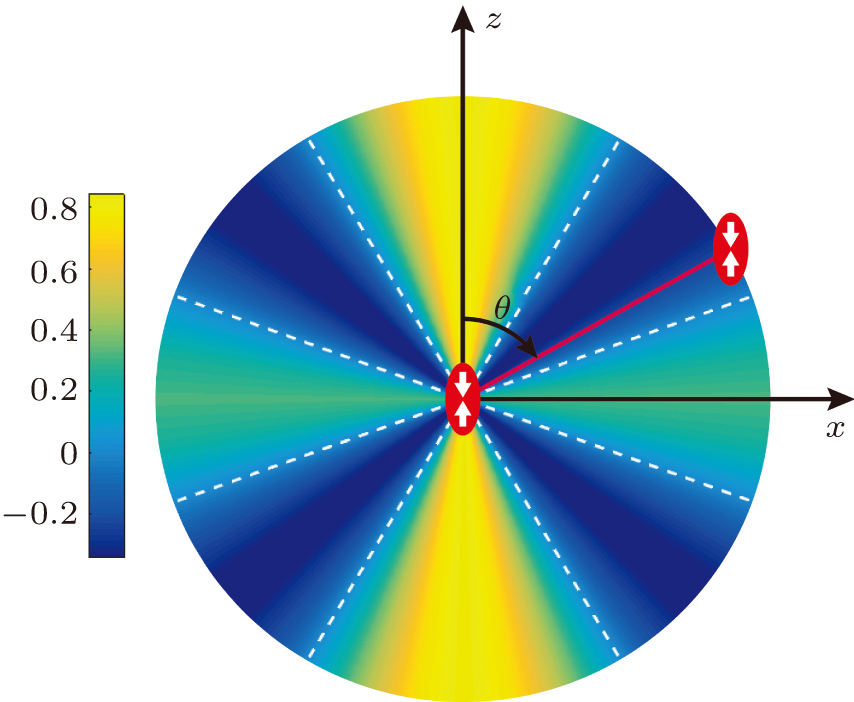
For two quadrupoles Θ₁ and Θ₂ with two molecular axes being along and , respectively, the QQI is^[38] 3 where r = |r|, , and ε₀ is the vacuum permittivity. To further simplify the QQI, we assume that all particles posses the same quadrapole moment Θ and molecular axes are polarized along the z axis by an electric field gradient.^[21] The QQI then reduces to 4 where θ is the polar angle of r and is the spherical harmonic.

In Fig. 1, we plot the angular dependence of V_qq(r). As can be seen, the QQI interaction is repulsive along both axial (θ = 0) and radial (θ = π/2) directions and it is most attractive along θ ≃ θ_m ≡ 49.1°. Compared to the dipolar interaction, the angular dependence of the quadrupolar interaction is more complicated. Moreover, the 1/r⁵ dependence on the inter-particle distance indicates that the QQI is a short-range interaction, while the DDI is a long-range one.

Fig. 1.

	Figure Option ViewDownloadNew Window
	Fig. 1. (color online) Angular dependence of the QQI, i.e., Y40(θ,φ). Positive (negative) value represents repulsive (attractive) region. Dashed lines mark the boundaries between the attractive and repulsive regions where the QQI vanishes.

It should be noted that, from the quantum mechanical point of view, because the quadrupole moment operator is of even parity, an atom with definite angular momentum quantum number J and magnetic quantum number M may carry a nonzero quadrupole moment. Consequently, one may effectively align the quadrupole moment with lights or magnetic fields to prepare the atoms in a particular angular momentum eigenstate, |J,M⟩, or their superposition.^[18,19]

We consider a trapped ultracold gas of N linear Bose molecules. In addition to the QQI [Eq. (4)] that was introduced in Section 2, we assume that molecules also interact via the contact interaction 5 where a₀ is the s-wave scattering length and m is the mass of the molecules. The total interaction potential then becomes 6 The confining harmonic potential is assumed to be axially symmetric, i.e., 7 where ω_⊥ and ω_z are the radial and axial trap frequencies, respectively. For convenience, we assume that the geometric average of the trap frequencies is constant. Consequently, the external trap is expressed as 8 where λ = ω_z/ω_⊥ is the trap aspect ratio.

Within the mean-field theory, a quadrupolar BEC is described by the condensate wave function Ψ(r,t) which satisfies the Gross–Pitaevskii equation (GPE) 9 where , , and g₀ and g_q characterize the strength of the contact and quadrupolar interactions, respectively. Here, for simplicity, we have introduced the dimensionless units: for length, ℏω_ho for energy, for time, and for wave function. Consequently, , , g₀ = 4πNa₀/a_ho, g_q = NΘ²/ , and are all dimensionless quantities. The rescaled wave function is now normalized to unit, i.e., . From the dimensionless equation (9), it can be seen that the free parameters of the system are the trap aspect ratio λ, the contact interaction strength g₀, and the quadrupolar interaction strength g_q. Given that we shall only deal with the dimensionless quantities from now on, the “bar” over all variables will be dropped for convenience.

The ground-state wave function can be obtained by numerically evolving Eq. (9) in imaginary time. The only numerical difficulty lies at the evaluation of the mean-field quadrupolar potential 10 Similar to the dipolar gases, can be conveniently evaluated in the momentum space by using the convolution theorem, i.e., 11 where and denote the Fourier and inverse Fourier transforms, respectively. Making use of the partial wave expansion , it can be easily shown that 12 where k = |k| and . Numerically, the evaluation of can be performed using the fast Fourier transform.

Finally, we fix the interaction parameters based on realistic systems. Since the s-wave scattering length is easily tunable through Feshbach resonance, here we shall only focus on the quadrupolar interaction strength g_q. The quadrupole moments of the metastable alkaline-earth and rare-earth atoms,^[39–43] and the ground-state homonuclear diatomic molecules^[44] can be calculated theoretically. In particular, for the Yb atom and homonuclear molecules, the quadrupole moment can be as large as 30 a.u.^[43,44] Therefore, for a typical configuration with N = 10⁴, Θ = 20 a.u., ω_ho = (2π) 1000 Hz, and m = 150 amu, we find g_q ≈ 66. As will be shown below, this QQI strength is large enough for experimental observations of the quadrupolar effects.

In this section, we investigate ground-state properties of the quadrupolar condensates. To easily identify the quadrupolar effects, we will focus on pure quadrupolar condensates by letting g₀ = 0. This reduces the control parameters to λ and g_q. We remark that, in the presence of the contact interaction, the results presented below remain quantitatively valid as long as g_q ≫ g₀.

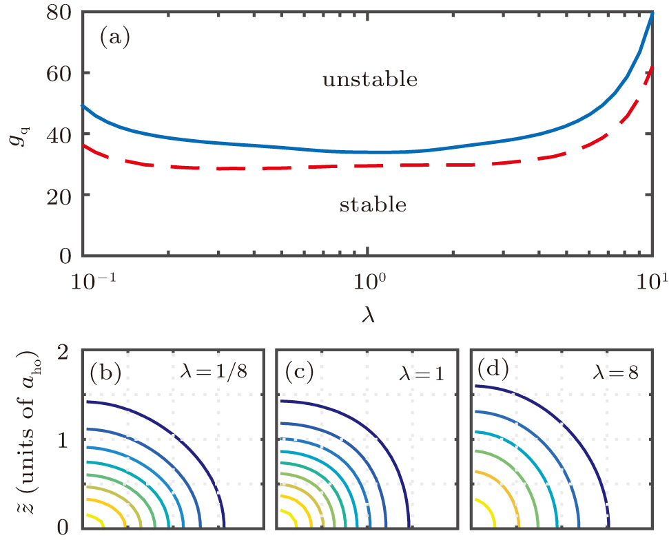
Since the QQI is partially attractive, stability is a particular important issue for the system. Numerically, it is found that, for a given λ, the condensate always becomes unstable when g_q exceeds a threshold value . In Fig. 2(a), we map out the stability diagram of a quadrupolar condensate on the (λ,g_q) parameter space, in which the solid line shows the critical QQI strength . The stability of a quadrupolar condensate strongly depends on the trap geometry. In fact, it becomes more stable for both highly oblate and elongated traps. This observation is in agreement with the angular distribution of the QQI shown in Fig. 1, as in both cases, the overall QQI is repulsive.

Fig. 2.

Figure Option ViewDownloadNew Window

Fig. 2. (color online) (a) Stability diagram on the (λ,gq) parameter space. The solid line is the critical QQI strength obtained via full numerical calculations, while the dashed line is obtained via Eq. (14) using condensate peak density along the solid line. Panels (b)–(d) show the contour plots of the condensate density for parameter sets (λ,gq) = (1/8,38), (1,33), and (8,52), respectively. Three triangles in panel (a) marks the positions of these parameter sets.

To gain more insight into the stability of the quadrupolar condensates, we consider a homogeneous quadrupolar condensate, for which the dispersion relation of the collective excitations is^[23] 13 where n is the density of the gas and all quantities are in dimensionless form under the units that were previously defined. Then, by noting that the minimum value of is , equation (13) leads to an analytical expression of the critical QQI strength 14 which suggests that a homogeneous condensate becomes unstable when . The dashed line in Fig. 2(a) represents the critical QQI strength . Here, for a given λ, the density n in Eq. (14) is taken as the numerically obtained peak condensate density corresponding to the parameters (λ,g_q) on the solid line of Fig. 2(a). As can be seen, there is only a small discrepancy between the analytic and numerical stability boundaries. The inequality equation (14) underestimates the critical QQI strength because the zero-point energy in the trapping potential is neglected when we use the homogeneous result for the dispersion relation.

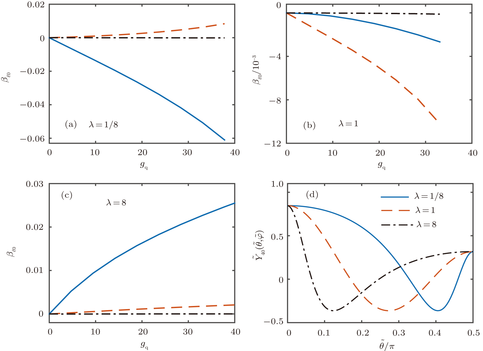
We now turn to study how the QQI deforms the condensates. Compared to dipolar gases whose deformation is essentially characterized by a single parameter, the condensate aspect ratio,^[45,46] the situation for quadrupolar condensate is more complicate. Because it is easier to visualize the deformation if the trapping potential is isotropic, we need to rescale the coordinates such that the isodensity surface of the condensate is a sphere in the absence of the QQI. For this purpose, we note that the condensate wave function at g_q = 0, 15 can be transformed into a spherically symmetric form by rescaling the coordinates according to , , and . This inspires us to consider the condensate density in the rescaled coordinates, i.e., 16 In Figs. 2(b)–2(d), we present the contour plots of under three different pairs of parameters. Careful examination of these contour lines reveals that the condensate is stretched mainly along the radial and axial directions for λ = 1/8 and 8, respectively. While for λ = 1, the condensate is stretched roughly along the direction that is most attractive for the QQI. To characterize the deformation quantitatively, we expand at a given radius into 17 where are the spherical coordinates for , β_ℓμ are the deformation parameters, and n₀ is determined by . In this work, is so chosen that n₀ is half of the peak condensate density. We note that because the ground-state wave function is axially symmetric, β_ℓμ is nonzero only if μ = 0.

Figures 3(a)–3(c) show the g_q dependence of the deformation parameters β_ℓ0 for ℓ = 2, 4, and 6 and for three different λ’s. In all three cases, β₆₀ are negligibly small. Furthermore, β₂₀ dominates in highly anisotropic traps and β₄₀ gives the largest contribution in isotropic potential, which is in agreement with the observation in Fig. 2. To understand these results, we express the angular dependence of the QQI, Y₄₀(θ,φ), in the rescaled coordinates 18 In Fig. 3(d), we plot for different λ’s. As can be seen, for λ = 1/8 and 8 the most attractive direction is shifted to and 0.12π, respectively. Therefore, one can naturally observe that the condensates are stretched along the radial and axial directions for λ = 1/8 and 8, respectively. We note that, compared to DDI, the deformation induced by QQI is much smaller. This can be attributed to the two features of the QQI. The complicated angular distribution of the QQI makes it difficult to induce a global deformation. Moreover, the short-ranged feature makes the condensate prone to collapse. Therefore, the strong interaction regime that may be required to generate large deformation is inaccessible.

Fig. 3.

	Figure Option ViewDownloadNew Window
	Fig. 3. (color online) (a)–(c) Deformation parameters βl0 versus QQI strength gq for ℓ = 2 (solid lines), 4 (dashed line), and 6 (dash–dotted lines). The trap aspect ratios are λ = 1/8 (a), 1 (b), and 8 (c). (d) Angular dependence of the QQI in the rescaled coordinates for different λ’s.

In Figs. 4(4) and 4(b), we plot the g_q dependence of the QQI energy, and the peak condensate density, n_p, respectively. As can be seen, the angular distribution of the density in an isotropic potential always makes the overall QQI attractive such that E_qq remains negative and n_p increases monotonically with g_q. Meanwhile, in highly anisotropic potentials, the angular dependence of the density is mainly determined by the trap, which, for both elongate and oblate traps, leads to overall repulsive QQI. Consequently, the peak density decreases with growing QQI strength in the small g_q region. For large g_q close to the stability boundary, the g_q dependence of n_q depends on the value of λ, which may exhibit distinct tendency.

Fig. 4.

	Figure Option ViewDownloadNew Window
	Fig. 4. (color online) Quadrupolar interaction energy (a) and condensate peak density (b) versus the QQI strength. The solid, dashed, and dash–dotted lines represent λ = 1/8, 1, and 8, respectively.

In conclusion, we have studied the ground-state properties of a trapped quadrupolar BEC. For the geometries of the ground states, we have quantitatively characterized different components of the deformation induced by QQI. In addition, we map out the stability diagram on the (λ,g_q) parameter plane. Finally, we point out that the QQI interaction strength required to induce the quadrupolar collapses is in principle accessible in, for example, a metastable Yb atom or homonuclear diatomic molecules, albeit the experimental realization of BECs of those atoms or molecules still remains challenging.