During the past several decades, the probability densities of an electron escaping from a photoionization process have been measured using a position-sensitive detector placed at a macroscopic distance.^[1–10] For the photoionization of atoms in the external field, the ionized electron is affected by both the external field and the long-range Coulomb field of the residual ion. Multiple classical paths are from the atom to any point in the classical allowed region on the detector, and the waves travelling along these paths produce an oscillatory structure in the electron probability density distribution.^[11–13] Since hydrogen has only one electron, which is the simplest atom, many researchers have studied the photoionization of the hydrogen atom in an external field. When the hydrogen atom is in a uniform electric field, the Stark Hamiltonian is exactly separable in terms of parabolic coordinates and its theoretical treatment is relatively simple.^[14–17] The photoionization cross section and the positions and widths of resonances were calculated and found to be in excellent agreement with the experimental results. In the early 1980s, Demkov et al.^[18] and Kondratovich and Ostrovsky^[19–21] proposed an experimental method to study the ionization of a hydrogen atom in an electric field. They found that when the hydrogen atom in a uniform electric field is photoionized by a laser beam with sharply defined frequency, the low-energy photoelectron waves can be emitted from the nucleus and are drawn toward a position-sensitive detector, which is located perpendicularly to the electric field. The electron probability density distribution on the detector is measured as a function of impact radius. An interference pattern which reflects the nodal structure of the quasibound atomic wave function will appear on the detector. This predication has been realized in a recent photoionization microscopy experiment by Stodolna et al.,^[22] who observed the nodal structure of the Stark state wave function at a microscopic distance.

In the theoretical aspect, Zhao and Delos studied the photoionization microscopy of a hydrogen atom in an electric field using both the semiclassical theory and the quantum mechanics method. First, they developed a semiclassical open orbit theory to study the dynamics of electron wave propagation in an electric field and calculated the electron probability densities on the detector plane.^[23] Then, they used the quantum-mechanical method to calculate the spatial distributions of electron probability densities for the same system.^[24] The correspondence of the quantum-mechanical results to the semiclassical open orbit theory suggests the correctness of the semiclassical method. Since the semiclassical open-orbit theory provides a clear and intuitive physical picture to explain the observed geometrical interference patterns in photoionization microscopy, many researchers have used this theory to study the photoionization of a hydrogen atom in other external fields, such as in the magnetic field, in parallel electric and magnetic fields, etc.^[25–27] However, as far as we know, all previous theoretical treatments were performed in the approximation of a uniform external field. As for the photoionization of Rydberg hydrogen atom in the non-uniform external fields, no report has been presented to date. In a recent study, Dumin studied the Stark effect in the strongly non-uniform electric field.^[28] In the study, the non-uniform electric field exerted on the excited electron can be considered as a gradient electric field. In 1999, Yang and Du studied the photodetachment cross section of H⁻ ion in a gradient electric field.^[29] Very recently, our group investigated the photo-detached electron flux distribution in a gradient electric field.^[30] In the case of the photodetachment, the escaping electron is subjected only to the gradient electric field. The number of the electron trajectories from the ion to any point on the detector is limited. However, for the photoionization of a hydrogen atom in the gradient electric field, the situation becomes much more complex. The escaping electron is affected by both the gradient electric field and the Coulomb field. The electron trajectory becomes more complex than that in the case of the photodetachment. An infinite number of classical trajectories will arrive at a given point on the detector plane, which causes a more complicated observable interference pattern in the photoionization microscopy.

In this paper, we study the electron probability density distribution for the Rydberg hydrogen atom in a gradient electric field on the basis of the photoionization microscopy for the first time; specifically we discuss the effects of the electric field gradient and the scaled energy on the photoionization microscopy interference patterns. By comparison with the photoionization of the hydrogen atom in an electric field,^[21] the electron trajectories in the gradient electric field will become chaotic and the number of the electron trajectories that can reach the detector plane becomes increased, which makes the interference pattern in the electron probability density distribution extremely complicated.

The rest of this paper is organized as follows. In Section 2, we describe the photoionization process of the Rydberg hydrogen atom in the presence of a gradient electric field, and put forward an analytical formula for calculating the electron probability density distribution on the detector plane. In Section 3, we calculate the electron probability density distribution on the detector plane, in particular we discuss the effects of the electric field gradient and the scaled energy on the electron probability density distribution. Finally in Section 4, we draw some conclusions from the present study in this paper. Scaled units are used in the paper unless otherwise specified.

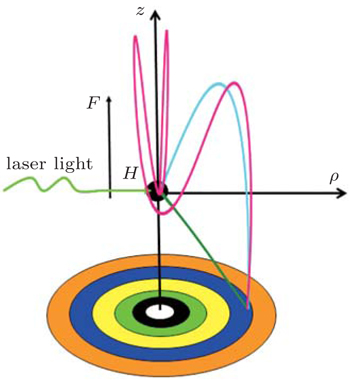
The schematic plot of the photoionization of a hydrogen atom in a gradient electric field is given in Fig. 1. Let the applied gradient electric field be in the z direction, which is given by F = F₀ + αz,^[29,31] where F₀ is the uniform background field and α is the electric field gradient in the z direction, which is a positive constant. A position-sensitive detector is placed perpendicularly to the z axis at the z = −z₀ plane, where z₀ is the distance between the hydrogen nucleus and the detector plane. The hydrogen atom lies at the origin of the coordinate system. When the hydrogen atom is ionized by a laser light, the ionized electron waves propagate outward from the nucleus in all directions, following classical trajectories. As the electron moves far from the nucleus, we can use the semiclassical approximation to construct the wave function.^[27] Owing to the influences of the gradient electric field and Coulomb field, more than two electron trajectories can reach the same point on the detector plane. The interference of the associated waves from the atom to any given point on the detector plane will produce an oscillatory pattern in the electron probability density distribution. A series of concentric interference fringes is schematically plotted on the detector plane as shown in Fig. 1.

Fig. 1.

	Figure Option ViewDownloadNew Window
	Fig. 1. Schematic description of the photoionization process of the hydrogen atom in a gradient electric field. The electric field F is along the z axis and the detector plane is perpendicular to the −z axis. A set of concentric interference fringes, which are caused by the interference of different electron trajectories arriving at the same point on the detector plane, are schematically plotted.

In cylindrical coordinates (ρ, z), the Hamiltonian governing the electron motion in the gradient electric field is

Owing to the cylindrical symmetry of the system, the z component of angular momentum is taken to be zero for simplicity. The potential-energy term is a combination of the Coulomb potential plus the gradient electric field, which can be expressed as^[29,31]

After transforming variables according to and ^[32] we obtain the transformed Hamiltonian (the tilde “∼” has been omitted) as follows:

From the above equation, we find that the scaled Hamiltonian depends only on scaled electric field gradient α and scaled energy ε, but not on the background electric field F₀.

In order to find the electron trajectories that have reached the detector plane, we should integrate the Hamiltonian motion equation. From Eq. (3), we find that there is a Coulomb singularity at the origin. Then we use the parabolic coordinates (u,v) and their conjugate momenta (p_u, p_v) instead of the cylindrical coordinates. The relations between the parabolic coordinates and the cylindrical coordinates are as follows:

A new scaled time variable τ is defined by dτ/dt = 1/(u² + v²). After introducing an effective Hamiltonian h = 2r(H − ε), we obtain

Let h = 0, the Hamiltonian (Eq. (6)) can generate the same trajectories as that for setting H = ε. Each electron trajectory can launch from the origin with the outgoing angle θ, which is defined as the angle between the initial velocity of the electron and the +z axis, and expressed as θ = tan⁻¹(ρ/z) = 2tan⁻¹(v/u). By numerically integrating the Hamiltonian motion equation, we can search out the electron trajectories that have arrived at the detector plane. Let the scaled energy ε = −0.1, the scaled electric field gradient α = 3.0, the detector is located at z = −0.5 plane, we plot some of the electron trajectories as shown in Fig. 2. These trajectories can be divided into different types. The first type of electron trajectory is usually emitted at large outgoing angles (θ > π/2) in a downhill direction. Under this condition, the initial velocity along the −z axis is large and the electric field force along the z axis plays a dominant role. Then after a short period of time, it reaches the detector without rotating in the ρ–z plane. This kind of orbit is called the direct trajectory,^[18] such as those depicted in Figs. 2(a) and 2(b). As θ decreases, the electron will leave the ion in an uphill direction. The Coulomb force and the electric field force have comparable magnitudes, the electron trajectory will rotate in the ρ–z plane. After a relatively long time, it will encircle the nucleus once or more times before it finally hits the detector. This kind of orbit is called the indirect trajectory. Figures 2(c)–2(h) belong to this kind of trajectory. As θ further decreases, the trajectory will become chaotic and stay close to the ion for a long time, the trajectories become much more complex.

Fig. 2.

	Figure Option ViewDownloadNew Window
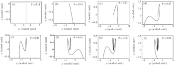
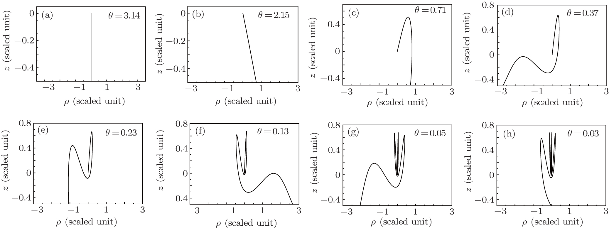
	Fig. 2. Some typical electron trajectories in the gradient electric field at scaled energy ε = −0.1, scaled electric field gradient α = 3.0, with the detector located at z = −0.5 plane. The initial outgoing angle is shown in each panel.

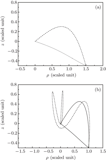
Through the calculation, we find that due to the combination of the electric field force and the Coulomb potential, more than one electron trajectory can arrive at a given point on the detector plane. In Fig. 3, we plot some of the electron trajectories that are emitted from the ion and arrive at a given point on the detector plane. Figure 3(a) shows two different electron trajectories arriving at the same point (1.5, −0.5) on the detector. In Fig. 3(b), three different electron trajectories can reach the same point (1.0, −0.5) on the detector.

Fig. 3.

	Figure Option ViewDownloadNew Window
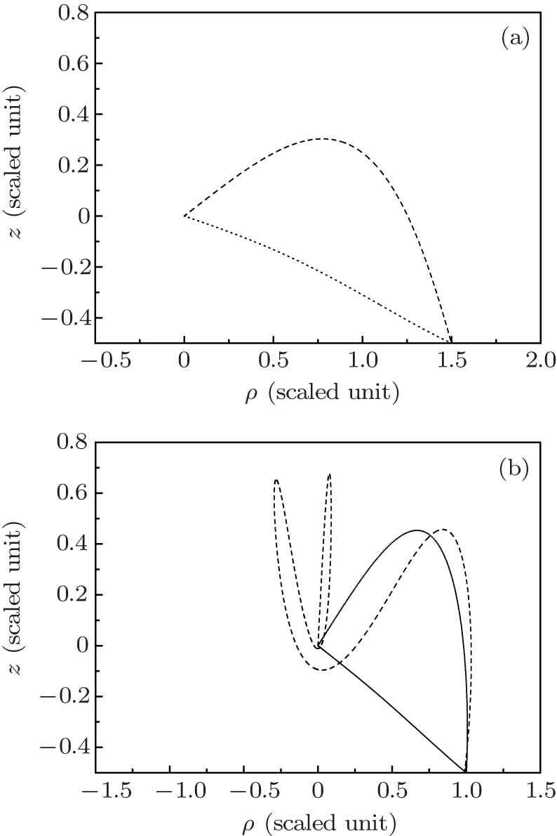
	Fig. 3. Some classical electron trajectories in the gradient electric field, hitting the same point on the detector. The scaled energy ε = −0.1, the scaled electric field gradient α = 3.0, the detector is located at z = −0.5 plane. Different trajectories are represented by different types of lines. The given point on the detector is as follows: (a) ρ = 1.5, z = −0.5; (b) ρ = 1.0, z = −0.5.

Next, we use the semiclassical approximation to construct the electron wave function. At a given point M(ρ,z₀) on the detector plane, the electron wave function corresponding to the j-th trajectory is denoted by ψ_j(ρ,z₀), whose magnitude and phase depend on its classical density A_j and phase factor χ_j:

Since more than one electron trajectory can arrive at a given point on the detector plane, the final wave function ψ_f(ρ,z₀) at point M(ρ,z₀) can be obtained by summing over all the possible trajectories as^[27]

The calculated radial electron probability density distribution at point M(ρ,z₀) is given by the following formula:

The first term on the right-hand side of Eq. (11) is the classical probability density distribution, and the second term represents the interference among different classical trajectories arriving at a given point on the detector.^[25,27]

By integrating the Hamiltonian motion equation (Eq. (6)) with the initial condition u(t = 0) = 0, v(t = 0) = 0, p_u(t = 0) = 2cos (θ/2), p_v(t = 0) = 2sin(θ/2), we can search out all the ionization trajectories of the Rydberg hydrogen atom in a gradient electric field. For different values of outgoing angle θ, the values of evolution time t taken for a trajectory to go from the ion to the detector plane are different. In this work, we stop the integration when the electron trajectory cannot reach the detector plane during a maximum period of time, T_max = 20 (scaled unit). For each electron trajectory, the outgoing angle θ, the impact point ρ on the detector and the Maslov index μ are recorded. Simultaneously, the classical action S is calculated.

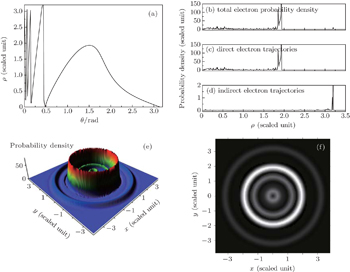
Firstly, we choose the scaled energy ε = −0.1, the scaled electric field gradient α = 3.0, the detector is located at z = −0.5 plane. Figure 4(a) shows a curve of the impact radius ρ at the detector plane versus the outgoing angle θ of the electron for the Rydberg hydrogen atom in a gradient electric field. From this figure, we find that the multiple classical electron trajectories emitted from the atom can impact the detector plane. The whole ρ–θ curve is divided into two different regions. Trajectories in a range with the outgoing angle 0.48 ≤ θ ≤ π can hit the detector directly without crossing the z axis; these trajectories are the direct ones. However, when the outgoing angle of the electron is limited in the region 0 ≤ θ ≤ 0.48, the electron will encircle the nucleus before it reaches the detector; these trajectories are the indirect ones. Once all the electron trajectories going from the atom to the detector plane are found, we can calculate the electron probability density distribution arising in the photoionization microscopy of a hydrogen atom in a gradient electric field. Figure 4(b) shows the variation of the two-dimensional electron probability density distribution with the impact radius ρ for the contribution of the total electron trajectories. Owing to the interference effect of different types of electron trajectories arriving at a given point on the detector plane, an oscillatory structure appears in the electron probability density distribution. Under this condition, the oscillatory structure is restricted in the region 0 ≤ ρ ≤ 3.20. The peak at about ρ = 1.85 means that the number of electrons that can reach the detector at this radius is the biggest. In order to have a clear insight into the building up of the interference pattern, the total electron probability density is broken down into the contribution of the direct electron trajectories and that of the indirect electron trajectories, which are shown in Figs. 4(c)–4(d). In this case, the direct trajectories correspond to the electrons with outgoing angle θ > 0.48 (see Fig. 4(a)); while the values of outgoing angle θ < 0.48 correspond to the trajectories of indirect electrons. From the calculation, we find that the contribution of the direct electron trajectories to the electron density probability plays a main role. As the launching angles for the indirect trajectories are small, this will lead to a small sinθ in the classical density. Thus, according to Eqs. (10) and (11), the contributions of indirect trajectories are very weak compared with those of the direct electron trajectories. In order to see the contributions of the indirect trajectories to the electron probability density, we change the scale of the coordinates to demonstrate the contribution of the indirect electrons trajectories clearly. To show the electron probability density distribution on the detector plane clearly, we further plot the three-dimensional probability density distribution on the detector plane, which is shown in Fig. 4(e). A series of interference rings appears in the electron probability density distribution. Different circular rings represent different electron probability density. Figure 4(f) gives the image plot of Fig. 4(e), which can be measured on the position-sensitive detector in the photoionization microscopy experiment. It is shown that the electron probability density distribution on the detector plane consists of a series of bright and dark concentric rings. The bright rings correspond to the constructive interference of different electron trajectories, while the dark rings correspond to the destructive interference.

Fig. 4.

Figure Option ViewDownloadNew Window

Fig. 4. The photoionization microscopy of the hydrogen atom in a gradient electric field, with scaled energy ε = −0.1, scaled electric field gradient α = 3.0, and the detector located at z = −0.5 plane. (a) The dependence of the impact position ρ at the detector plane on the initial outgoing angle θ; (b) the two-dimensional electron probability density distribution on the detector plane, corresponding to the contribution of the total electron trajectories; (b) the electron probability density caused by the direct electron trajectories; (c) the electron probability density caused by the indirect electron trajectories; (e) the three-dimensional electron probability density distribution on the detector plane; (f) the image of Fig. 4(e).

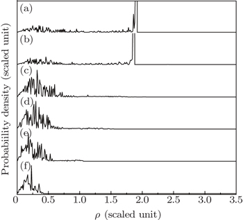
Secondly, we fix the scaled electric gradient and the position of the detector plane to be α = 3.0 and z₀ = −0.5, respectively. Then we discuss the variation of the photoionization microscopy of the hydrogen atom in gradient electric field with scaled energy. Under this condition, the saddle point energy is ε_s ≈ −0.87. As the excitation energy of the electron is smaller than the saddle point energy, no electron trajectory can escape from the nucleus and reach the detector. In the following calculation, we choose the scaled energy varying from ε = 0.0 to ε = −0.74. Figure 5 shows the relation of the impact radius ρ on the detector plane with the initial angle θ at which the electron trajectory is launched for different scaled energies. Figure 5(a) shows the ρ–θ curve with the scaled energy ε = 0.0. From this figure, we find that an infinite number of trajectories can reach the detector. Trajectories in a range with the outgoing angle 0.44 < θ < π are the direct ones and those in a range with the outgoing angle 0 < θ < 0.44 are the indirect ones. With the decrease of the scaled energy, the range of the outgoing angle for the direct trajectory becomes narrow. Besides, the maximum impact radius that the electron can reach decreases correspondingly. For example, in Fig. 5(a), the maximum impact radius that the electron can reach is ρ_max = 3.58. As the scaled energy decreases to ε = −0.74, the maximum impact radius that the electron arrives at the detector decreases to ρ_max = 1.39. The range of the direct electron trajectories is only limited in a region 0.81 ≤ θ ≤ π. In addition, this figure suggests that as the scaled energy is close to the ionization threshold, ε = 0.0, nearly all electron trajectories with the outgoing angle 0 < θ ≤ π can strike the detector. However, with the decrease of the scaled energy, a critical angle θ_c appears in the ρ–θ curve. The electron trajectories leaving the ion with an initial angle larger than that critical angle arrive very quickly at the detector, but those leaving with an initial angle below that critical angle can stay forever in the vicinity of the ion. For example, in Fig. 5(d), ε = −0.6, the critical angle θ_c = 0.44, all the electron trajectory with the outgoing angle less than θ_c will never escape from the Coulomb attraction nor the electric field force and cannot reach the detector within the given time. As we further reduce the scaled energy, the critical angle becomes enlarged. As the scaled energy is very low, the number of indirect electron trajectories arriving at the detector plane becomes small.

Fig. 5.

	Figure Option ViewDownloadNew Window
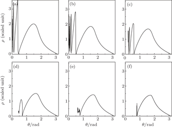
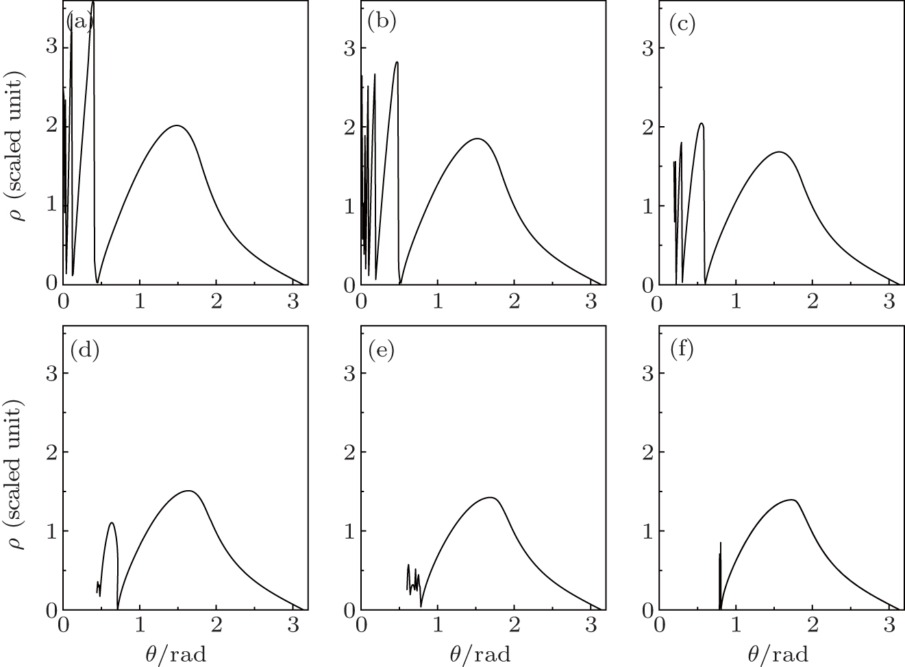
	Fig. 5. Variations of the impact radius ρ on the detector plane with the outgoing angle of the electron at different scaled energies. The detector is located at z = −0.5 plane. The scaled electric field gradient is α = 3.0. The scaled energies are (a)ε = 0; (b) ε = −0.2; (c) ε = −0.4; (d) ε = −0.6; (e) ε = −0.7; (f) ε = −0.74 respectively.

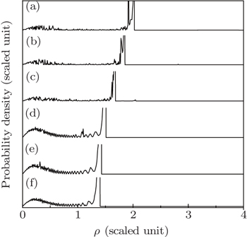
In Fig. 6, we calculate the two-dimensional electron probability density distributions arising in photoionization microscopy of a hydrogen atom in a gradient electric field for different scaled energies. From this figure, we find oscillatory structures appear in the electron probability density distributions, which can be considered as a consequence of the interference effect caused by different types of electron trajectories arriving at a given point on the detector plane. Figure 6(a) shows the electron probability density distribution with the scaled energy ε = 0.0. Under this circumstance, the number of the electron trajectories arriving at the detector plane is large. Both the direct electron trajectories and the indirect ones can arrive at a given point on the detector plane, which makes the oscillatory structure in the electron probability density distributions complex. The maximum impact radius that the electron can reach is ρ_max = 3.58, the oscillatory structure is restricted in a large region 0 < ρ < 3.58. With the decrease of the scaled energy, the number of the indirect electron trajectories arriving at the detector plane decreases and the oscillating region in the electron probability density distributions reduces. For example, as the scaled energy ε = −0.74, the oscillatory structures arise primarily from the interference of the direct electron trajectories, and a two-term interference pattern plays an important role. The electron probability distribution is only restricted in a small region 0 < ρ <1.39. In order to have a clear insight into the building up of the interference pattern, we plot the three-dimensional probability density distribution on the detector plane at different values of scaled energy, ε = −0.2, ε = −0.4, ε = −0.6, and ε = −0.7. The calculation results are shown in Fig. 7. The panels in the left column correspond to the three-dimensional probability density distributions on the detector plane, while the panels in the right column show the corresponding image plots. The electron probability density distribution on the detector plane consists of a series of interference rings. In the same circular ring, the probability density is the same. With the decrease of the scaled energy, the radius of the ring decreases correspondingly. As the scaled energy is relatively large, ε = −0.2, the maximum impact radius on the detector is also large, which makes the radius of the outmost ring in the image plot large (see Fig. 7(a)). The maximum impact radius on the detector decreases with the decrease of the scaled energy, which makes the radius of the outmost ring in the image plot smaller and the disk in the image plot is reduced (see Figs. 7(b)–7(d)).

Fig. 6.

	Figure Option ViewDownloadNew Window
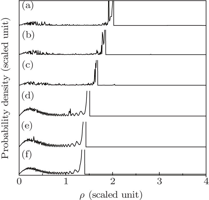
	Fig. 6. Variations of the electron probability density distribution on the detector plane with impact radius ρ at different scaled energies. The detector is located at z = −0.5 plane. The scaled electric field gradient is α = 3.0. The scaled energies are (a) ε = 0, (b) ε = −0.2, (c) ε = −0.4, (d) ε = −0.6, (e) ε = −0.7, and (f) ε = −0.74 respectively.

Fig. 7.

Figure Option ViewDownloadNew Window

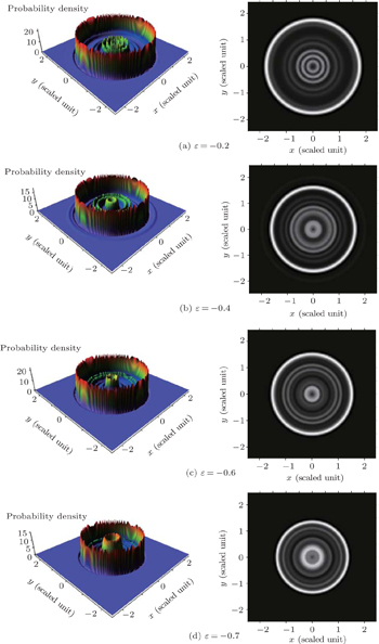
Fig. 7. Three-dimensional electron probability density distributions on the detector plane at different scaled energies. The detector is located at z = −0.5 plane and the scaled electric field gradient α = 3.0. The panels in the left column correspond to the three-dimensional probability density distributions on the detector plane, while the panels in the right column show the corresponding images. The scaled energy is given in each plot.

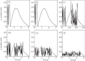
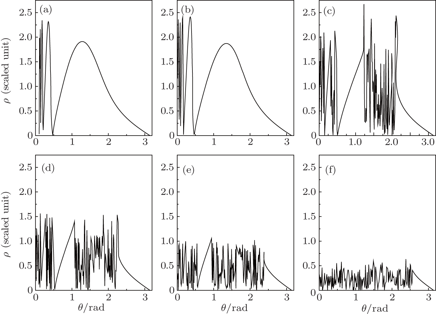
Thirdly, we fix the scaled energy and the detector plane and show the influence of the gradient electric field on the photoionization microscopy interference pattern of the Rydberg hydrogen atom. In the calculation, we set ε = −0.1, z₀ = −0.5. Figure 8 shows the variations of the final position ρ at the detector plane versus outgoing angle θ for different gradient electric fields. Figure 8(a) shows the ρ–θ curve with the scaled electric field gradient α = 0.0, which is similar to that for the photoionization of the Rydberg hydrogen atom in a uniform electrical field. From this figure, we find not all the electron trajectories with the initial angle 0 ≤ θ ≤ π can arrive at the detector plane. The electron trajectories with the outgoing angle 0 < θ < 0.10 will never reach the detector and will stay close to the ion forever. Only those electron trajectories with the outgoing angle above 0.1 can arrive at the detector plane. The trajectories in a range with the outgoing angle 0.10 < θ < 0.47 are the indirect ones and those in a range with the outgoing angle 0.47 < θ < π are the direct ones. The maximum impact radius that the electron can reach is ρ_max = 2.31. With the increase of the electric gradient, the effect of the electric field force caused by the gradient electric field becomes significant. The number of the electron trajectories arriving at the detector plane increases and the electron trajectories will become chaotic. The ρ–θ curve becomes complicated and exhibits fractal structure as well as a certain self-similarity, which is similar to the epistrophic self-similarity structure when treating the escape-time dynamics in the ionization of atoms in external fields.^[33,34] The reason can be explained as follows: According to the theory of electromagnetic fields, the influence of a varying electric field can be considered as a magnetic field. From Eq. (2), we find that the effect of the gradient electric field on the electron is similar to that of a magnetic field perpendicular to the z axis. Therefore, the gradient electric field will restrict the electron moving in the ρ–z plane. The gradient electric field causes the electron to oscillate more rapidly than a pure electric field. The larger the strength of the electric field gradient, the smaller the impact radius that the electron can reach on the detector plane. If the electric field gradient is very big, the electric field force becomes strong. Then after a short period of time, the electron will hit the detector plane, which causes the maximum impact radius that the electron can reach the detector plane to become much smaller, as we can see from Figs. 8(c)–8(f) clearly.

Fig. 8.

	Figure Option ViewDownloadNew Window
	Fig. 8. The ρ–θ curves for the photoionization of the Rydberg hydrogen atom in different gradient electric fields. The detector is located at z=-0.5 plane. The scaled energy is ε = −0.1. The scaled electric field gradients are (a) α = 0.0, (b) α = 1.0, (c) α = 6.0, (d) α = 8.0, (e) α = 10.0, and (f) α = 13.0.

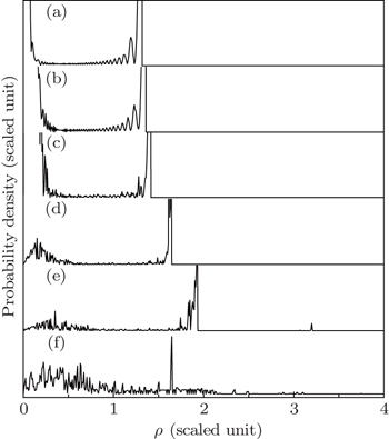
Figure 9(a) shows the variation of the electron probability density distribution in a uniform electrical field, ε = −0.1, z₀ = −0.5. Under this condition, the electric field gradient α = 0.0, only the background uniform electric field can influence the electron motion. The maximum distance that the electron can reach on the detector plane is large, which makes the oscillating region in the electron probability density distributions spread widely.

Figures 9(b)–9(f) show the electron probability density distributions in different gradient electric fields. Their background uniform electric field is the same as that in Fig. 9(a). The oscillatory structures in the electron probability density have a great difference from that in a uniform electrical field. With the increase of the electric field gradient, the effect of the gradient electric field plays an important role. The maximum impact radius decreases, which causes the oscillating structure in the electron probability density distribution to be restricted only in a small region. For example, when the scaled electric field gradient α = 13.0 (Fig. 9(f)), the maximum impact radius ρ_max = 0.63, and the oscillating region in the electron probability density distributions is restricted only in the region 0 < ρ <0.63.

Fig. 9.

	Figure Option ViewDownloadNew Window
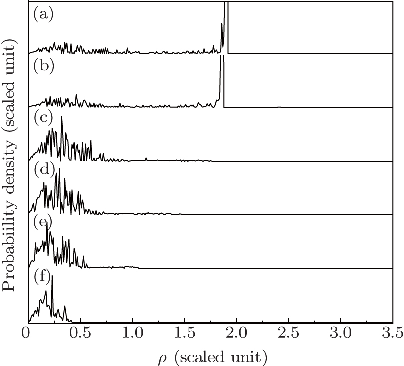
	Fig. 9. Electron probability density distributions for the photoionization of the Rydberg hydrogen atom in different gradient electric fields. The detector is located at z = −0.5 plane. The scaled energy is ε = −0.1. The scaled electric field gradients are (a) α = 0.0, (b) α = 1.0, (c) α = 6.0, (d) α = 8.0, (e) α = 10.0, and (f) α = 13.0, respectively.

Finally, we investigate the change of the photoionization microscopy for the Rydberg hydrogen in a gradient electric field with the position of the detector plane. Suppose that the scaled energy ε = −0.1 and the scaled electric field gradient α = 3.0. Figure 10 shows the change of the electron probability density distribution for the Rydberg hydrogen in a gradient electric field with the position of the detector plane. Figure 10(a) shows the electron probability density distribution with the detector located at z₀ = −0.01 plane. We find that the oscillatory structure is restricted in a small region 0 < ρ < 1.31. The oscillatory structure caused by the interference of the direct electron trajectories plays an important role. With the increase of the distance from the ion to the detector plane, the number of the electron trajectories arriving at the detector plane becomes increased, which makes the oscillatory structure in the electron probability density distribution much more complicated. The interference effects caused by the direct and indirect electron trajectories dominate in the probability density distribution. In addition, the electron probability density distribution on the detector plane becomes widely spread as the distance from the ion to the detector plane increases. For example, in Fig. 10(f), the detector is placed at z₀ = −0.8 plane, we find the oscillatory structure is spread in the region 0 < ρ < 3.99. According to the scaled transformation, if we take the uniform electric field strength F₀=10v/cm, then the position of the detector will be located at z₀ = −0.96 μm. The oscillatory structure in the electron probability density distribution is spread in the region 0 < ρ < 4.79 μm. Given the present state of the electric field and the position of the detectors, the calculated structures is observable in an actual experiment. Therefore, our study will be useful for guiding the future experimental research on the photoionization microscopy of the Rydberg atom in the presence of an external field.

Fig. 10.

	Figure Option ViewDownloadNew Window
	Fig. 10. Variations of the electron probability density distribution for the Rydberg hydrogen in a gradient electric field with the position of the detector plane. The scaled energy is ε = −0.1. The scaled electric field gradient is α = 3.0. The positions of the detector plane are (a) z0 = −0.01, (b) z0 = −0.05, (c) z0 = −0.1, (d) z0 = −0.3, (e) z0 = −0.5, and (f) z0 = −0.8, respectively.

We performed a semiclassical calculation of the photoionization microscopy of the Rydberg hydrogen atom in a gradient electric field, and investigate the interference patterns in the photoelectron probability density distribution on a detector plane. The influence of the gradient electric field on the electron dynamics is discussed in great detail. Our study suggests that by comparison with the scenario of the photoionization of Rydberg hydrogen atom in a uniform electric field, the number of the indirect electron trajectories arriving at the detector plane becomes increased, which makes the oscillatory patterns in the photoelectron probability density distribution complicated. As the electric field gradient is relatively small, the maximum impact radius that the electron can arrive at the detector plane is large, which makes the oscillating region in the probability density distributions restricted in a large region. With the increase of the electric field gradient, it will restrict the electron motion, which makes the maximum impact radius that the electron can reach the detector plane smaller and the oscillating region in the probability density distributions narrowly spread. In addition, the oscillatory structures in the electron probability density distribution are dependent on the scaled energy sensitively. Through our research, we predict that if the external electric field strength and the position of the electron detector plane are reasonable, the photoionization microscopy interferograms are observable in an actual experiment. We hope that our results will be useful for guiding experimental studies of the photoionization microscopy of Rydberg atoms in a non-uniform external field.