Cheng Zhao-Hua†, He Wei, Zhang Xiang-Qun, Sun Da-Li, Du Hai-Feng, Wu Qiong, Ye Jun, Fang Ya-Peng, Liu Hao-Liang. Manipulating magnetic anisotropy and ultrafast spin dynamics of magnetic nanostructures . Chinese Physics B, 24(7): 077505
Permissions
Manipulating magnetic anisotropy and ultrafast spin dynamics of magnetic nanostructures
Cheng Zhao-Hua†, He Wei, Zhang Xiang-Qun, Sun Da-Li, Du Hai-Feng, Wu Qiong, Ye Jun, Fang Ya-Peng, Liu Hao-Liang
State Key Laboratory of Magnetism, Institute of Physics, Chinese Academy of Sciences, Beijing 100190, China
*Project supported by the National Basic Research Program of China (Grant Nos. 2015CB921403, 2011CB921801, and 2012CB933101) and the National Natural Science Foundation of China (Grant Nos. 51427801, 11374350, 51201179, and 11274361).
Abstract
We present our extensive research into magnetic anisotropy. We tuned the terrace width of Si(111) substrate by a novel method: varying the direction of heating current and consequently manipulating the magnetic anisotropy of magnetic structures on the stepped substrate by decorating its atomic steps. Laser-induced ultrafast demagnetization of a CoFeB/MgO/CoFeB magnetic tunneling junction was explored by the time-resolved magneto-optical Kerr effect (TR-MOKE) for both the parallel state (P state) and the antiparallel state (AP state) of the magnetizations between two magnetic layers. It was observed that the demagnetization time is shorter and the magnitude of demagnetization is larger in the AP state than those in the P state. These behaviors are attributed to the ultrafast spin transfer between two CoFeB layers via the tunneling of hot electrons through the MgO barrier. Our observation indicates that ultrafast demagnetization can be engineered by the hot electron tunneling current. This opens the door to manipulate the ultrafast spin current in magnetic tunneling junctions. Furthermore, an all-optical TR-MOKE technique provides the flexibility for exploring the nonlinear magnetization dynamics in ferromagnetic materials, especially with metallic materials.
PACS:
75.78.–n; 75.40.Gb; 76.50.+g; 75.70.–i
Keyword:
magnetic anisotropy; ultrafast spin dynamics; magnetic nanostructures
During the past two decades, continuous miniaturization has been driving the data-storage technology to the nanometer scale. The rapid development in fabrication and applications of nanostructured magnetic devices drives us to understand the magnetism of low-dimensional systems. By virtue of their extremely small sizes, nanomagnets possess significantly different properties from their parent bulk materials. The quantum tunneling of magnetization in nanomagnets is a prototype of the quantum effect at the macroscopic scale and could be utilized for quantum information and computation. The theorem of Mermin and Wangner is always employed to discuss low-dimensional magnetic properties.[1] According to this theorem, an infinite d-dimensional lattice of localized spins cannot hold long range magnetic order (LRMO) at any finite temperature if d < 3 and the effective exchange interaction among the spins is isotropic in spin space and finite range.[1] By contrast, the LRMO in a low-dimensional magnetic system can be achieved via incorporating anisotropy, including non-isotropic exchange constants, dipole– dipole interaction, single-ion anisotropy, etc. into the model.[2] Therefore, magnetic anisotropy can be regarded as one of the origins of long range magnetic order in low-dimensional magnetic systems.
Magnetic anisotropy also plays a vital role in determining the magnetic and spin-dependent transport properties for magnetically hard materials, magnetically soft materials, high-frequency magnetic materials, ultra high density magnetic recording media, and spintronic materials. In the case of a homogenous ellipsoid, Brown’ s theorem states that the coercivity Hc satisfies[3]
where α is the microstructural parameter, Ku is the uniaxial magnetic constant, Ms is the saturation magnetization, and Neff is the effective demagnetizing factor. For a permanent magnet, a strong uniaxial magnetic anisotropy is the prerequisite for high coercivity (Fig. 1).
Fig. 1. Magnetic hysteresis loop for magnetic material.
For ultra high density magnetic recording media and spintronic materials, the following trilemma of magnetic recording must be grappled with. (i) Achieving high medium signal noise ratio (SNR) requires the utilization of small grains. (ii) The energy that can be stored in one grain is KuV, where Ku is the uniaxial magnetic constant and V is the grain volume. This energy competes against the thermal energy kBT and must be large enough to prevent spontaneous magnetization reversals, which would lead to thermal decay and eventually superparamagnetism. Small grains have energy barriers (KuV) that are too small to ensure the thermal stability of the recorded information (Fig. 2). Scaling of the bit size in the conventional magnetic recording media is becoming increasingly difficult due to the superparamagnetic limit. In principle, the magnetic energy KuV can be maintained for smaller grain volumes if the uniaxial magnetic constant Ku is increased accordingly. (iii) An increase in the uniaxial magnetic constant Ku increases the required write field beyond the capability of available head materials. Consequently, one approach to extend the superparamagnetic limit of the media to 1 Tb/in2 and beyond is to increase the uniaxial magnetic constant Ku as large as KuV ≥ 40kBT.[4]
Fig. 2. Sketch of superparamagnetism of ultrahigh density magnetic recording media.
In addition to the strength of magnetic anisotropy, its symmetry is also important for high-frequency magnetic materials. The miniaturization and rapid increase in frequencies of electric devices require that magnetic materials possess high resonance frequency, large permeability, and low magnetic loss. The natural resonance frequency fr is generally regarded as the upper limit frequency, i.e., the cut-off frequency, of magnetic materials. For the traditional spinel ferrites with cubic symmetry, the natural frequency is proportional to the magnetic anisotropy constant, fr = γ Ku/π Ms, and the ac susceptibility is , where γ is the gyromagnetic ratio and μ 0 is the permeability of free space. Therefore, the product of the susceptibility and the resonance frequency of one high-frequency magnetic material is proportional to its saturation magnetization, i.e., the Snoek limit, [5]
It is a great challenge to increase both resonance frequency and permeability simultaneously due to Snoek’ s limit. Alternatively, for the magnetic materials with different anisotropy fields Ha1 and Ha2 in the hard plane and the easy plane, the product of the initial rotational permeability μ i and the resonance frequency satisfies fr[6]
From Eq. (3), one can conclude that the product of the initial rotational permeability and the resonance frequency of magnetic materials with different anisotropy fields can be enhanced by a factor of compared with the magnetic materials with cubic symmetry.
1.2. Methods of manipulating magnetic anisotropy
In the case of a bulk magnetic material, the overall magnetic anisotropy, which is governed mainly by magnetocrystalline anisotropy, cannot be tuned greatly if its crystal symmetry is fixed. In contrast, for the magnetic nanostructures, we have more freedom to manipulate the magnetic anisotropy via changing the symmetry of magnetic dots, the interspace of wires, or the thickness of films. There are various techniques to manipulate the magnetic anisotropy of magnetic nanostructures. In this review, we just focus on magnetic anisotropy manipulation via substrate decoration and oblique deposition of Fe and Co on Si(111) substrates.
Surface-supported quasi one-dimensional (Q1D) magnetic nanostructures such as atomic chains, nanostripes, and nanowires have often been used as model systems to investigate low-dimensional magnetism. For this purpose, vicinal metallic substrates are commonly used.[7– 12] The atomically flat terraces separated by steps are generally used as templates for preparing various self-organized nanostructures, including regular arrays of nanodots, [13] nanostripes, [7, 8] atomic wires, [11] and ultrathin films.[9] Furthermore, the terraces can be employed to confine magnetic nanodot assemblies and form one-dimensional (1D) quantum-well states.[14– 18] For these low-dimensional magnetic materials, novel electronic structures and magnetic properties often emerge from the interplay between quantum confinement and broken symmetry. As a result, the magnetic anisotropy of the magnetic nanostructures can be drastically manipulated by the stepped surfaces. Recently, we observed tunability in both the magnetic anisotropy and the magnetic coupling of Fe nanodots on a curved Cu(111) substrate by varying the terrace width.[19]
The growth and the magnetic properties of single crystal Fe film on Si(111) surface have been investigated owing to its application in integration of magnetic devices in Si-based technology and new opportunities in spintronics.[20– 27] The Si(111) substrate has often been selected to obtain different stepped surfaces.[28, 29] Compared to metallic substrates, it is convenient to obtain a clean Si substrate surface, and the surface morphology can be manipulated by different treating processes.[30– 32] As a result, the magnetic anisotropy of magnetic nanostructures can be drastically manipulated by the stepped surfaces.
In addition to the stepped surfaces, the surface morphology has a significant effect on magnetic anisotropy.[33, 34] The interaction between the deposited atoms and the atoms on the surface modifies the trajectory of the deposited atoms, which is called the steering effect, and causes an inhomogeneous distribution of adatoms.[35, 36] In oblique-incidence deposition, such a steering effect is important and generally introduces grains that are elongated perpendicular to the plane of the incident flux direction. These elongated grains always lead to an in-plane uniaxial magnetic anisotropy (UMA) when depositing magnetic materials.[37] Therefore, an in-plane uniaxial magnetic anisotropy can be induced by oblique deposition.
1.3. Brief introduction of ultrafast spin dynamics — femtomagnetism
The current trend in the spintronic devices with a faster response demands the study of the magnetization dynamics of magnetic nanostructures on very small time scales.[38] Femtosecond laser pulses offer the intriguing possibility to probe a magnetic system on a time scale that corresponds to the (equilibrium) exchange interaction, responsible for the existence of magnetic order, while being much faster than the time scale of spin-orbit interaction (1– 10 ps) or magnetic precession (100– 1000 ps). Since the laser-induced ultrafast demagnetization was first observed in Ni films, [39] significant progress has been made in exploring the coupling between the laser excitation and the spin system.[40– 47] Despite being the subject of intense research for about two decades, the underlying mechanisms that govern the demagnetization remain unclear. The corresponding mechanism has its origin in relativistic quantum electrodynamics, beyond the spin– orbit interaction involving the ionic potential. Laser-induced femtosecond magnetism or femtomagnetism opens a new frontier for a faster magnetic storage device, but probing such a fast magnetization change is a big challenge. The understanding of the ultrafast demagnetization process is a very important issue, not only for investigating the coupling between spin, electron, and lattice in a strongly out-of-equilibrium regime, but also for the potential application of spintronic devices in the terahertz regime.[48]
1.4. Determination of magnetic anisotropy by magneto-transport method
To date, various methods, such as magnetic hysteresis loop measurement, torque measurement, [49] ferromagnetic resonance (FMR), [23] rotational magneto-optic Kerr effect (ROT-MOKE), [50] and magnetic transverse biased initial inverse susceptibility and torque (TBIIST), [51] have been developed to determine the magnetic anisotropy constants. Since the coherent domain rotation magnetization reversal for ultrathin film does not always occur, especially when the applied field is lower than the saturation field, the detailed information regarding the magnetic anisotropy cannot be distinguished precisely from the magnetization hysteresis loops.
Alternatively, the magneto-transport method has been proved to be an ideal probe of magnetic anisotropy constants in the thin single layer films by anisotropic magnetoresistance (AMR).[52– 58] The schematic configuration of the sample and the coordination in AMR measurements are illustrated in Fig. 3. AMR can determine the anisotropy field strength by realization of a coherent magnetization reversal (Stoner– Wohlfarth like) (Fig. 4). This can be achieved by applying a sufficiently large field to guarantee a true single-domain rotation. The AMR can be expressed as
where φ M is the angle between the magnetization M and the current flow I, and R∥ and R⊥ are the resistances at φ M = 0° and φ M = 90° , respectively.
Owing to the magnetic anisotropy, M is no longer kept along with the external field H during rotation, i.e., φ M < φ H, where φ H is the angle between the magnetic field H and the current I. Therefore, the AMR curves do not follow the cos2φ H relationship. On the basis of the angle difference between φ H and φ M, we can further calculate the magnetic torque L(φ M) = μ 0MsH sin(φ H − φ M) curves at different external fields. In order to compare the magnetic torques at different fields, the normalized magnetic torque l(φ M) = L(φ M)/μ 0MsH = sin(φ H − φ M) can be derived (Fig. 5). Finally, the uniaxial magnetic anisotropy and first- and second-order magnetocrystalline anisotropy constants are precisely obtained by fitting the normalized magnetic toque curves.
Fig. 5. Normalized magnetic torque curves obtained from AMR curves.
2. Manipulating magnetic anisotropy of magnetic nanostructures
2.1. Step-induced uniaxial magnetic anisotropy of quasi-one-dimensional Fe chains on Pb/Si(111) substrate
Nowadays the magnetism of low-dimensional systems is among the most interesting subjects in which the nanostructures and the magnetic anisotropy are related. Theoretically, the ferromagnetism cannot exist in an isolated 1D chain with only isotropic finite-range exchange interactions unless the symmetry is broken in the presence of magnetic anisotropy, dipolar, and/or RKKY interaction.[1, 2] Experimentally, the fabrication of the reduced symmetry systems presents a challenge with regard to which there has been real progress recently: to grow 1D nanostripes or nanowires of transition metals on stepped surfaces by molecular beam epitaxy (MBE). In pioneering experiments, Hauschild et al. produced ferromagnetic Fe stripes on W(110) with the in-plane magnetic easy axis perpendicular to the stripes due to the long-range dipolar interaction.[7] Shen et al. reported that the Fe stripes grown on stepped Cu(111) behaves with the easy magnetization normal to the surface at low coverage (< 0.8 ML) within the short-range ferromagnetic order explained by Ising spin blocks.[8, 9] Li et al. also observed step-decoration Fe stripes on Pd(110) with its easy magnetization axis along the surface normal.[10] Gambardella et al. demonstrated the increased magnetic anisotropy energy (MAE) of Co monatomic chains on Pt(997) in the case of reducing the size of nanostructures, [11] while Cheng et al. investigated the contribution of the polarization of the proximal Pt to the magnetic anisotropy of Fe stripes on Pt(997).[12]
Here, we report our fabrication of low-dimensional Fe nanodots grown on Pb (111) substrate by MBE. From the scanning tunneling microscopy (STM) image (Fig. 6), one can find that the symmetries of the nanodots on the terrace and on the step of the Pb(111) surface are quite different. Iron nanodots distribute randomly on the terrace, while forming quasi-one dimensional chains on the step. These results suggest that one can control the growth and the magnetic properties of Fe nanodots via substrate decoration.
Fig. 6. STM image of Fe nanodots on Pb(111) substrate.
Due to the difficulty in obtaining uniform steps and controlling their terrace width in the vicinal Pb(111) substrates, and for transport and spintronic applications, [27] it is highly desirable to grow the magnetic nanowires on Si substrates so that a natural integration with Si-based devices can be achieved. A well-known obstacle is the formation of silicides. We explore a method of fabricating the nanodots and nanochains on 0.1° and 4° miscut Si(111) substrates, respectively, using atomically flat Pb films as a buffer layer (Fig. 7). Step widths of about 200 nm and 10 nm are achieved, respectively. Moreover, the Pb buffer layer can prevent interdiffusion of Fe/Si.
Fig. 7. Schematic configuration of the growth of Fe nanodots and nanochains on Pb/Si(111) substrate with different miscut angles.
Similar to the results of Fe nanodots on Pb(111) substrate, STM images (Fig. 8) indicate that Fe nanoclusters distribute randomly on the 0.1° miscut Si(111) substrate. On the other hand, quasi-1D nanowires are formed by coalescence of bcc Fe islands along the edge steps of the Pb/Si(111) surface. The edges of the wires are rough due to the 3D fractal shape of the Fe islands, as the results of the lattice mismatch and the large surface energy difference between Fe and Pb.[59] The distance between the wires just equals the terrace width of the stepped Pb/Si(111) film. It is not like Fe stripes grown on Cu(111), in which Fe atoms have a tendency toward growth across the steps of Cu(111).[9] The 3D-shaped Fe islands first located on the Pb/Si(111) steps at low coverage facilitate the nucleation of Fe atoms deposited afterward along the steps, decrease the diffusion across the steps, and smooth the edge of the wires at higher coverages.
Fig. 8. STM images of Fe nanodots (a) and nanochains (b) on 0.1° and 4° miscut Si(111) substrates.
In order to characterize the magnetic anisotropy, representative magnetic hysteresis loops with polar, longitudinal, and transverse surface magneto-optical Kerr effect (SMOKE) were measured. In the polar geometry, the applied field is normal to the surface. In the longitudinal geometry, the applied field is parallel to the surface along the step direction of the Pb films. In the transverse geometry, the applied field is also parallel to the surface but normal to the step direction. The applied field is in the plane of incidence in all three configurations. On the 0.1° miscut Si(111) substrate, SMOKE hysteresis loops indicate that the Fe nanodots are almost isotropic in the Si(111) surface (not shown). In contrast, for the Fe nanochains with coverage up to 1.7 ML, the longitudinal Kerr loop shows a nearly rectangular shape loop, while the polar and transverse Kerr loops indicate sheared loops without remanence (Fig. 9). We attribute this to the induced magnetic anisotropy associated with the step edges, [60] and the contribution of dipolar interaction between the Fe chains and/or islands inside the chain.
Fig. 9. SMOKE hysteresis loops measured in (a), (d) polar, (b), (e) longitudinal, and (c), (f) transverse geometries for Fe nanochains on 4° miscut Si(111) substrates with different coverages.[61]
FMR has been established as one of the most powerful techniques to investigate static and dynamic magnetic properties.[62] In addition to in situ SMOKE measurements, an ex situ FMR measurement could allow us to determine the easy magnetization direction as well as the magnetic anisotropy constant. Figures 10(a) and 10(b) show the angular dependences of in-plane and out-of-plane FMR spectra taken at room temperature (RT) for the 1.7 ML Fe chains, respectively. The in-plane and out-of-plane FMR spectra each consist of two peaks (labeled by P1 and P2). The black circles in Figs. 10(c) and 10(d) show the angular variation of in-plane and out-of-plane resonance fields for the P1 peak. (The P2 peak shows resonance fields that do not change with angles. It is a paramagnetic resonance (PMR) peak existing in the background spectra.) This implies that the sample has uniaxial in-plane symmetry, because it shows three peaks in angular dependence in the plane of the film if cubic anisotropy of Fe is present.[63] Considering the SMOKE data, one assumes that only the Zeeman energy, the in-plane uniaxial magnetic anisotropy energy, and the demagnetization energy are to be taken into account for the free energy density of the system for 1.7 ML Fe/Pb/Si (Ref. [63], and references therein). Hence, the in-plane and out-of-plane resonance fields Hres can be calculated by using the following equations derived from the Landau– Lifshitz equation without damping:[62]
where (θ , φ ) and (θ H, φ H) are the angles for the magnetization and the applied resonance field, respectively, and θ and φ correspond to the out-of-plane orientation with the film normal and the in-plane orientation perpendicular to the wire direction; γ = gμ B/ħ is the gyromagnetic ratio; 4π Meff is the effective magnetization; and Ku is the in-plane uniaxial anisotropy constant. The lines obtained by fitting the experimental data with Eqs. (5)– (8) are also shown in Figs. 10(c) and 10(d). The in-plane uniaxial magnetic anisotropy is found to display a dominant uniaxial symmetry, and its easy axis is along the chain direction, consistent with the SMOKE measurements. The parameters g, 2Ku/Ms, 4π Meff are estimated from the fit lines with g = 2.03 and 2Ku/Ms = 15 mT, which proves that the P1 peak is the ferromagnetic resonance (FMR) peak. Considering the fact that each Fe 3D random island inside the wire contains 6000 atoms on average, one would expect these Fe islands to have a magnetization close to the bulk value. Taking the bulk value Ms = 1.7 × 10⁶ J/m3, the overall in-plane uniaxial anisotropy constant Ku can be obtained as 1.3 × 10⁴J/m3.
Fig. 10. Angular dependence of the out-of-plane (a) and in-plane (b) FMR spectra taken at RT. The FMR resonance fields as a function of the out-of-plane and in-plane field orientations are shown in panels (c) and (d), respectively. The circles are experimental data and the solid lines represent the theoretical fitted curves.[61]
Both FMR and SMOKE measurements indicate that the magnetization easy axis of the Fe chains on Pb/Si is along the wires’ direction, from which it might be inferred that the shape magnetic anisotropy, originating from magnetostatic interactions among the Fe islands, is the dominant factor that determines the magnetic properties of the Fe chains. In order to verify the prediction and quantitatively describe the system, the Monte Carlo method is used to investigate the magnetic properties of the system. In the present simulation, we adopt the approach developed by Beleggia et al. to treat the effect of the shape magnetic anisotropy on the magnetostatic coupling among Fe islands.[64, 65] The 1.3 ML Fe nanowires, seen in Fig. 11(a), are approximately composed of irregular Fe islands. For simplicity, in the calculation of magnetostatic energy among Fe islands, we ignore the size distribution of the Fe islands and regard the islands as having an elliptic cylinder shape with a = 2.0 nm, b = 2.5 nm, and h = 0.6 nm on average, where a and b are lengths of the axes of the Fe island (along the x and y directions, respectively), and h is the height of the Fe island (along the z direction), as shown in Fig. 11(e). As the Fe deposition proceeds, the islands mainly enlarge two dimensionally by branching out, and coalescence of islands first occurs along the y direction due to the limitation of the Pb step, as shown in Fig. 11(b) with 1.7 ML Fe. In Fig. 11(d), we schematically show the variation of the islands with increasing Fe coverage. In Fig. 11(c), ax and ay are defined as the interwire distance and the interparticle distance in one nanowire, respectively. The averaged values ⟨ ax⟩ = 6 nm and ⟨ ay⟩ = 5 nm come from the statistics of STM images. In the Monte Carlo simulation, the parameters of Fe islands for three typical coverages are used: (i) Θ = 1.0 ML (separate islands), (ii) Θ = 1.3 ML (critical point), (iii) Θ = 1.7 ML (overlapping islands).
Fig. 11. STM images of Fe chains at (a) 1.3 ML and (b) 1.7 ML. (c) Schematic diagram of the model. (d) Schematic evolution of the growth of Fe island: the initial nucleation (yellow area), growth (blue area), and coalescence (gray area). (e) 3D diagrammatic sketch of one Fe island.[66]
Figures 12(a) and 12(b) show the calculated magnetic hysteresis loops at coverage Θ = 1.3 ML (T = 150 K) and Θ = 1.7 ML (T = 290 K), respectively. The corresponding experimental results are displayed in Figs. 12(c) and 12(d). In both cases, it is seen that the easy axis is along the y axis and no magnetic hysteresis loops are observed in the other two directions, which shows good agreement between the experimental and the calculated data. It is also shown that the calculated loops have a good square degree, which suggests that the magnetic switching is finished by coherent rotation of the magnetization.
Fig. 12. (a) and (b) Representative calculated hysteresis loops for the system with coverage Θ = 1.3 ML and 1.7 ML. (c) and (d) The corresponding SMOKE curves with the same external parameters.[66]
2.2. Contribution of magnetocrystalline anisotropy to Fe nanostructures on Si(111) surface
In the previous work, the quasi-one-dimensional Fe chains on the 4° miscut Si(111) substrate with a Pb film as a buffer layer were fabricated, and an in-plane uniaxial magnetic anisotropy was induced by the stepped surface. However, due to the large lattice mismatch (aFe = 2.87Å , aPb = 3.5 Å ) and the vastly different surface free energy between Fe and Pb (σ Fe = 2.48 J/m2, σ Pb = 0.5 J/m2), Fe nanoclusters tend to form a polycrystalline structure, and the effect of magnetocrystalline anisotropies of Fe on the magnetic properties of the system is eliminated. Now, we report the structure and the magnetic properties of single crystal Fe film with thickness of 45 ML grown on vicinal Si(111) substrates using a flat ultrathin p(2 × 2) iron silicide seed layer. The epitaxial growth mode between the Fe films and the substrate is preserved in this system, providing the opportunity of investigating the influence of magnetocrystalline anisotropies on the magnetic properties of the system.[67]
In order to prevent the Fe/Si intermixing, an iron silicide buffer layer was first grown by deposition of 1.5 ML Fe followed by annealing to 700 K for 10 min. An iron film with a thickness of 45 ML was deposited on the iron silicide template; STM images of the iron silicide film on the 0.1° and 4° miscut Si(111) substrates are displayed in Figs. 13(a) and 13(c). The vicinal structure of the bare Si(111) substrate is well revealed by the buffer layer of iron silicide. The corresponding 2× 2 LEED pattern is displayed in the inset of Fig. 13(a). This film comprises bunches of steps separating the flat 2× 2 reconstructed terraces. The bunched steps are parallel to each other and regularly distributed on the surface. An atomically resolved 2× 2 reconstructed surface is shown in the insets of Figs. 13(a) and 13(c). Each protrusion in the figure is a Si adatom.
Fig. 13. STM images of the iron silicide films and Fe film on the 0.1° (a), (c) and 4° (b), (d) miscut Si(111) substrates.[67, 69]
Figures 13(b) and 13(d) display the STM images of the Fe film with thickness of 45 ML grown on the p(2× 2)(111)/Si(111) surface. The morphology of the Fe film is characterized by self-organized non-uniform Fe grains preferentially aligned along the step direction. Due to the decoration of the step, Fe nanodots and nanochains are formed on the wider and the narrower terraces, respectively. The epitaxial relationships among the Fe layer, the iron silicide template, and the Si substrate are[68] Fe(111) | | p(2× 2)(111) | | Si(111) and Fe[-1-12] | | p(2× 2) [-1-12] | | Si[11-2].
The total free energy density of the system with the external field H is[23]
where the first term is the Zeeman energy, is the unit vector of the magnetic vector, and Ms is the saturation magnetization of Fe (taken as the bulk value 1.74 × 10⁶ A/m); the second and the third terms are the cubic magnetocrystalline anisotropy energy, α i represent the directional cosines of the magnetic vector with respect to the cubic axes [100], [010], and [001], K1 and K2 are the first two cubic magnetocrystalline anisotropy constants; the last three terms sequentially refer to the uniaxial magnetic anisotropy energy, the surface magnetic anisotropy energy, and the out-of-plane demagnetization energy; Ku, Ks, and are the corresponding magnetic anisotropy constants. The unit vector with its orientation along the step direction represents the direction of the easy axis of the uniaxial magnetic anisotropy; and are the unit vectors normal to the (111) plane and the vicinal (111) film plane, respectively. It should be noted that the unit vector is perpendicular to the vicinal plane, unlike a simple flat thin (111) film sample with its hard axis of the out of plane demagnetization energy perpendicular to the (111) crystallographic plane.
The angular dependence of magnetocrystalline anisotropy energy of cubic symmetry is illustrated in Fig. 14. The energy of magnetocrystalline anisotropy in the Fe(111) surface can be written as [51]
Fig. 14. Angular dependence of magnetocrystalline anisotropy energy with cubic symmetry.
We can find that the K1 energy term is invariable and the K2 energy term is sixfold symmetry in the Fe(111) plane. The experimental in-plane magnetic hysteresis loops for several angles (φ = 0° , 45° , 70° , 90° ) are shown in Fig. 15. The loops show approximately the same shape in the angle range 0° ≤ φ ≤ 40° . A magnetic hysteresis loop of the hard axis is observed in the angle φ = 90° . Owing to the weak coercivity, the symmetry of magnetocrystalline anisotropy is unclear from the magnetization measurement.
Fig. 15. In-plane magnetic hysteresis loops for several azimuthal angles.[67]
In order to understand the contribution of magnetocrystalline anisotropy, the magnetic anisotropies of the sample were measured by FMR. The in-plane FMR spectra with different azimuthal angles are displayed in the left panel of Fig. 16(b). The azimuthal angle dependence of the resonance field is shown in the right panels of Figs. 16(a) and 16(b) (green circles) for Fe nanodots and nanochains on 0.1° and 4° miscut Si(111) substrates, respectively. The cubic anisotropy contribution to the sixfold anisotropy for a flat (111) film is evident. As for the Fe nanochains on 4° miscut Si(111) substrates, four maxima and minima of the resonance fields are observed within the azimuthal angle range 0° ≤ φ ≤ 360° . This indicates that the in-plane magnetic anisotropy is the superposition of a fourfold and a uniaxial contribution. Fitting the experimental data using Eq. (9) and the standard FMR conditions yields the parameters K1 = 4.5 × 10⁴ J/m3, K2/K1 = 0.04, Ks/Kd = 0.09, and Ku = 9.2 × 10³ J/m3.
Fig. 16. Left: angular dependence of the in-plane FMR spectra taken at RT: (a) Fe nanodots on 0.1° and 4° ; (b) miscut Si(111) substrates. Right: experimental (green circles) and fitted (red line) curves of the relations between the resonance field and the rotated angle for in plane configurations, the calculated curve without the effect of uniaxial magnetic anisotropy for flat (111) plane: black lines, vicinal plane: blue lines.[67, 69]
We first consider the flat Fe(111) film without uniaxial magnetic anisotropy. It is known that the easy axis induced solely by the first order magnetocrystalline anisotropy is along the ⟨ 100⟩ direction. However, the effective out of plane demagnetizing field forces the magnetic moment of the system to lie in the (111) plane. Despite (Kd − Ks)≫ K1, the competition of the effective out of plane demagnetizing field and the first order magnetocrystalline anisotropy field results in a small deviation of magnetization with respect to the Fe (111) plane in the resonance condition. As a result, the in plane resonance field displays sixfold symmetry with the easy axis along the ⟨ 11-2⟩ directions for a positive K1 . According to the expression of the second cubic energy in the (111) film, E2 = K2 (1 + cos 6φ )/108, [51] the positive value of K2 corresponds to the easy axes along the six equivalent ⟨ -110⟩ directions. This is opposite to the effect of the first cubic magnetocrystalline anisotropy. Thus, the sixfold symmetry of the resonance field in the flat Fe(111) film, illustrated in the right panel of Fig. 16(b) (black lines), should be displayed under the influence of the effective out of plane demagnetization energy and the first two cubic magnetocrystalline anisotropies’ energy by means of the numerical calculation.
For the Fe films on the 4° miscut Si(111) substrate, the direction of the hard axis corresponding to the demagnetizing field of the film is slightly tilted by 4° along the [11-2] direction from the (111) plane. Compared with the case of a flat (111) plane, a relatively large deviation of magnetization with respect to the Fe (111) plane is induced. On the other hand, the cubic anisotropy’ s contribution to the sixfold anisotropy for a flat (111) film is very small and easily hidden (the variation of the resonance field for a perfectly aligned (111) film is less than 1 mT). In this case, small misorientations are sufficient to reduce the sixfold symmetry to fourfold, resulting in variations of the resonance field much larger than that in a (111) plane, as shown in the right panel of Fig. 16(b) (blue lines) by the numerical calculation. Finally, a twofold symmetry of the in plane resonance field, originating from the uniaxial magnetic anisotropy, is superimposed upon the fourfold one.
2.3. Effect of miscut angle on magnetic anisotropy in Fe nanostructures on Si(111) surface
In the case of a bcc Fe film grown on Si(111) substrate, the sixfold symmetry of magnetic anisotropy energy exists only when magnetization is confined strictly in the Fe(111) plane. A small structural modification is sufficient to destroy the sixfold symmetry as a result of the contributions from magnetic anisotropy energies.[23, 24] In the previous work, we observed that the sixfold symmetry of the in-plane resonance field for the Fe(111) film was changed into the superposition of a fourfold and a twofold contribution due to the presence of atomic steps of the vicinal substrate. Furthermore, we also observed some difference between ferromagnetic resonance (FMR) results and magnetization measurements. FMR results demonstrated that the azimuthal angular dependence of the in-plane resonance field has a sixfold symmetry with a weak uniaxial contribution, while the remanence of the hysteresis loops displays a twofold symmetry.[69] Therefore, the analysis of the magnetic anisotropy and magnetization reversal should be carried out carefully for Fe(111) films on Si(111) substrate.
Figures 17(a) and 17(b) present the angular dependence of the first- and the second-order magnetocrystalline anisotropy energy terms in the Fe(111) plane along [11-2] with various miscut angles, where K1 = 4.5 × 10⁴ J/m3 and K2 = 0.05K1.[69] We can find that the K1 energy term is invariable (solid line circle in Fig. 17(a)) and the K2 energy term is sixfold symmetric exactly in the Fe(111) plane, i.e., miscut angle β = 0° . However, the K1 energy term can be changed to have a fourfold symmetry by a slight misorientation from the (111) plane, i.e. β ≠ 0° . Figure 17(b) demonstrates that the symmetry of the K2 energy term keeps unchanged.
Fig. 17. Angular dependence of magnetocrystalline anisotropy energies. First (a) and second (b) order magnetocrystalline anisotropy energy terms for various miscut angles.[70]
In order to investigate the effect of tiny variations of miscut angles on the fitting parameters, we illustrate in Fig. 18 the fitted magnetic anisotropy constants for various miscut angles β from − 0.30° to 0.30° . It is noteworthy that a tiny variation of miscut angle β has no effect on the values of K2 and Ku (Fig. 18(a)), whereas it significantly affects the fitted values of the first-order magnetocrystalline anisotropy K1 (Fig. 18(b)).
Fig. 18. The fitted magnetic anisotropy constants K2 and Ku (a), and K1 (b) for various miscut angles β from − 0.30° to 0.30° .[70]
We find that the resistances of the Si substrate with and without the iron silicide buffer layer, which are almost the same, are somewhat larger than the resistance of the Fe ultrathin film. Furthermore, the Si substrate and the iron silicide buffer layer do not contribute to AMR. Therefore, the metallic Fe single crystal film grown on an iron silicide buffer layer and Si(111) surface with iron silicide provides an ideal system to perform AMR measurements.
Figure 19(a) shows the angular dependence of the in-plane AMR with different applied fields. The external magnetic fields are larger than the saturation field to guarantee a true single-domain rotation and eliminate the ordinary magnetoresistance effect. During the rotation of the sample, the AMR values show an oscillating behavior between the maximum value R∥ and the minimum value R⊥ . However, owing to the magnetic anisotropy, the magnetization M is no longer kept along with the external field H during rotation, i.e., φ M < φ H. Therefore, the AMR curves do not follow the cos2φ H relationship. The correlation between φ H and φ M can be obtained and is plotted in Fig. 19(b).
Fig. 19. In-plane AMR curves at different curves and the correlation between φ H and φ M . (a) Angular dependence of the in-plane AMR, and (b) the correlation between φ H and φ M at different fields.[70]
On the basis of the angle difference between φ H and φ M, we can further calculate the magnetic torque L(φ M) = μ 0MsH sin(φ H − φ M) at different external fields from Fig. 19(b). In order to compare the magnetic torques at different fields, the normalized magnetic torque l(φ M) = L(φ M)/μ 0MsH = sin(φ H − φ M) is introduced. As shown in Fig. 20(a), the normalized magnetic torque curves exhibit different shapes with different external fields H. In the equilibrium state, the torque acting on M due to H is equal in magnitude to the torque due to the magnetic anisotropies of the sample. Since the demagnetization field is normal to the Si(111) plane, its contribution to the magnetic torque is zero. According to Eq. (9), the normalized magnetic torque can be written as
Fig. 20. Normalized magnetic torque curves. (a) Normalized magnetic torque curves superposed by the first- and the second-order magnetocrystalline anisotropies and uniaxial anisotropy at different fields and (b) the normalized torque contributed only by the first- and the second-order magnetocrystalline anisotropies at field of 2 mT; the solid lines are fitting curves. For comparison, the normalized magnetic torque curves are also plotted in panel (a).[70]
Although the value of Ks(∼ 106 J/m3) is far larger than that of Ku (∼ 102 J/m3) for ultrathin Fe film, [67, 69] we can calculate from Eq. (10) that the value of torque contributed by Ks is at least two orders of magnitude smaller than that contributed by Ku. Therefore, the contribution of the surface anisotropy constant to the torque can be neglected.
It is obvious from Eq. (11) that the magnetic torque shows a superposition of two-, four-, and six-fold magnetic anisotropies from the step-induced uniaxial magnetic anisotropy Ku, the first-order magnetocrystalline constant K1, and the second-order magnetocrystalline anisotropy constant K2, respectively. The twofold symmetry disappears gradually with increasing external field H, suggesting that the strength of Ku is very weak. Therefore, in order to distinguish the contribution of Ku, the external field H should be kept slightly larger than the saturation field.
From Eq. (11), we can easily find that the normalized torque is significantly affected by the substrate’ s miscut angle β . The tendency of the anisotropy energy is complicated. We can find that the fourfold anisotropy energy changes significantly (Fig. 17(a)), while the six-fold anisotropy energy almost does not change with the miscut angle β (Fig. 17(b)). In the case of β = 0, the K1 term is zero. Usually the miscut angle of the substrate cannot be neglected, and thus the contribution from the first-order magnetocrystalline anisotropy constant in the vicinal (111) plane must be taken into account.
2.4. Tuning magnetic anisotropies of Fe ultrathin films on Si(111) substrate via direction variation of heating current
We have fabricated quasi 1D magnetic nanodot assemblies on vicinal Si(111) surface with relatively large miscut angles (∼ 4° ). Although both the magnetic anisotropy and the magnetic coupling of Fe nanodots can be achieved on a curved Cu(111) substrate by varying the terrace width, [19] the terrace width of these stepped substrates cannot be tuned easily once the miscut angle is fixed, which causes difficulty in investigating the effect of the terrace width on the magnetic properties by using identical substrates. Here, we adopted a novel method to tailor the terrace width of Si(111) substrates via controlling the direction of direct heating current passing through the sample. The magnetic anisotropy of the corresponding epitaxial Fe films grown on these Si(111) surfaces was continuously tuned.
Figure 21(a) schematically illustrates the configuration of the substrate treatment and the preparation process for these Cu/Fe/FeSi2/Si(111) samples. During the direct current heating treatment, [71] the current passed through the substrate, and the direction of current changed from being parallel to the step to being perpendicular. Figure 21(b) shows a coordinate system used in the magneto-optical Kerr effect (MOKE) measurements and the subsequent data simulation. The ex situ magnetization hysteresis curves were determined in the longitudinal MOKE geometry at different sample azimuthal angles φ . The azimuthal angle φ denotes the angle of the external magnetic field with respect to the surface step (Si [1-10]).
Fig. 21. Schematic configuration of the sample preparation and MOKE measurement, and STM images of sample surface. (a) Schematic configuration for treating substrate with controllable heating current and film preparation process. (b) Coordinate system used in the MOKE measurements and the subsequent data simulation. (c)– (f) STM images of clean surfaces on four Si(111) substrates I– IV with different widths of the terrace. The arrows indicate that the direction of the heating current changes continuously on each sample, which induces the variation of the width of the surface steps. (g), (h) STM images of 20 ML Fe films on p(2× 2)/Si(111) of samples I and IV, with the corresponding small scale images in the lower right corner. Typical LEED patterns are illustrated in the insets of panels (c) and (g).[72]
The large scale STM images in Figs. 21(c)– 21(f) demonstrate the atomically flat Si(111) surfaces of four samples I– IV with different terrace widths. The direction of heating current for each sample is denoted by the arrows in these images. The substrate of sample I was heated with the current parallel to the surface steps. The Si(111)-7× 7 reconstructed surface with the terrace width of 230 ± 30 nm was obtained as shown in Fig. 21(c). The Si(111)-7× 7 reconstructed surfaces for all four samples were measured by LEED. For samples II– IV, the angles between the heating current and the steps vary from 30° to 90° , resulting in a decrease of the terrace width. The corresponding terrace widths are dI = 100± 20 nm, dIII = 80± 20 nm, and dIV = 45± 15 nm, respectively (Figs. 21(d)– 21(f)).
The variation of terrace width of Si(111) substrate with heating current direction can be explained by the surface electromigration of Si adatoms.[31, 32] The step bunching due to heating by direct current has been well documented for the Si(111) surface with 1° miscut angle.[31, 32] It was observed that the step bunching was influenced by annealing temperature and the direction of current flow respectively. However, the effect of heating current direction either parallel or perpendicular to the step on the terrace width is not well understood yet. Here, we tuned the step morphologies by annealing vicinal Si(111) at a fixed temperature while adjusting the applied electric field from parallel to perpendicular to the step. When the Si(111) substrates were treated by direct current heating, the electric field, in addition to the heating temperature, influences the surface morphology. The Si adatoms would be driven by an electromigration force, where the electric field is applied on the Si adatoms, and qa is the effective charge of the Si adatoms. The electromigration force could drive the Si adatoms to flow on the surface along the direction of the electric field. When the direct current was applied parallel to the step (θ = 0° ), the Si adatoms would flow along the edge without changing the step density. Thereby, the widest terrace was achieved (Fig. 1(c)). On the other hand, when the direct current was applied perpendicular to the step (θ = 90° ), Si adatoms driven by the largest electromigration force perpendicular to the terrace edge, the adatoms would diffuse along the electric field and form the narrowest terrace, as shown in Fig. 21(f).
Within the framework of the surface electromigration model, a scaling law was derived[32]
where l is the average terrace width, N is the number of atoms in one step height, and F is the electromigration force perpendicular to the steps. Parameters α and q are positive exponents which vary for different systems and heating methods. For our samples with single atomic steps, equation (11) is simplified. Using the experimental data of samples II– IV, the value of parameter q = 1.1 is obtained. For sample I, when the electromigration force F perpendicular to the step is smaller than a critical value, the surface terrace will be stable and not become wider.
Figures 21(g) and 21(h) display the surface morphology of 20 ML iron film deposited on the FeSi2 p(2× 2)(111)/Si(111) surface of samples I and IV, respectively. The epitaxial growth of bcc α -Fe film is verified by the LEED pattern (inset of Fig. 1(g)). Due to the small grains of Fe with the surface fluctuation of 2.4± 0.3 nm, the single atomic steps become hardly visible. From the high resolution STM images in the lower right corners of Figs. 21(g) and 21(h), we can observe that the terrace width has no obvious influence on the grain size and shape.
The longitudinal MOKE measurements were performed with applied magnetic field at various orientation φ for each sample as illustrated in Fig. 21(b). Representative magnetic hysteresis loops measured by ex situ MOKE are displayed in Fig. 22. The variation of hysteresis loops with φ indicates in-plane magnetic anisotropy. For sample I, the hysteresis loops varied significantly. However, no loops with the normalized remanence close to 1 or 0 were found at any azimuthal angle φ . As shown in Fig. 22(a), the hysteresis loop with the largest and the smallest normalized remanence Mr/Ms = 0.782 and Mr/Ms = 0.365 appear at φ = 30° and φ = 60° , respectively, indicating that a sixfold magnetic anisotropy exists in this sample. The difference in hysteresis loops for φ = 30° and φ = 90° suggests that an additional magnetic anisotropy is superimposed. For the other three samples, rectangular hysteresis loops with Mr/Ms ≈ 1 and sheared loops without remanence were found at φ = 0° and 90° , respectively (Figs. 22(b)– 22(d)).
Fig. 22. Experimental and simulated magnetic hysteresis loops. Typical in-plane magnetic hysteresis loops at different azimuthal angles of samples I– IV ((a)– (d)) characterized by MOKE. Samples II– IV ((b)– (d)) exhibit standard easy and hard hysteresis loops at φ = 0° and 90° . The corresponding simulated hysteresis loops at the hard axis (red lines) are displayed in panels (b)– (d).[72]
For a comprehensive description of the in-plane magnetic anisotropy of these four samples, the normalized remanence Mr/Ms as a function of azimuthal angle φ of each sample is shown in Fig. 23. The complicated symmetry of magnetic anisotropy is observed in sample I from Fig. 23(a). The angular dependence of the normalized remanence with eight maxima can be explained well by the superposition of a sixfold and a UMA contribution. The UMA with the easy axis parallel to the steps makes the normalized remanence near φ = 0° generally larger than that around φ = 90° . Moreover, the sixfold magnetocrystalline anisotropy of Fe(111) film modifies the UMA to generate six other peaks at φ = 30° , 90° , 150° , 210° , 270° , and 330° , respectively. As displayed in Figs. 23(b)– 23(d), the other three samples exhibit similar twofold symmetric curves of the angular dependence of the normalized remanence. The peak width of the curves at φ = 0° increases with decreasing terrace width, suggesting that the UMA enhances and consequently conceals the weak sixfold magnetocrystalline anisotropy.
Fig. 23. Angular dependence of the normalized remanence Mr/Ms, obtained from the experimental hysteresis loops. Sample I shows a UMA superimposed on a weak sixfold anisotropy, and samples II– IV display a gradually enhanced UMA with the sixfold anisotropy almost concealed.[72]
Our work suggests that the magnetic anisotropy of Fe film on Si(111) substrate can be flexibly tuned by direct heating current. This finding opens a new avenue to manipulate the magnetic anisotropy via decorating the atomic steps of substrates, which can enrich our capacity of fabricating magnetic nanostructures and manipulating the magnetic properties for potential applications.
2.5. Tuning magnetic anisotropy of obliquely deposited Co/Si(111) films
Besides controlling the growth and magnetic properties of Fe nanodots via substrate decoration, oblique incidence deposition is an effective technique to introduce an in-plane UMA. We fabricated Co film on Si(111) substrate by oblique incidence deposition using a molecular beam epitaxy (MBE) system with a base vacuum of 10− 10 mbar by using electron gun evaporation at room temperature. A nominal thickness of 10 nm Co film was deposited on Si(111) substrates at an angle of 60° with respect to the surface normal and with azimuth along the y direction, i.e., perpendicular to the surface steps on the substrates, as shown in Fig. 24(a). For comparison, another 10 nm thick Co film was fabricated by normal incident deposition with the same growth rate. The STM image in Fig. 24(b) shows the surface of the oblique deposited sample. The clear grains are elongated perpendicular to the incident plane of the atomic flux and form a stripe structure with root mean square (RMS) roughness of 0.65 nm. However, for the normal incidence deposited Co film, the STM image shown in Fig. 24(c) demonstrates that the grain distribution on the film surface is isotropic and the RMS roughness is much less (∼ 0.12 nm) than that in the obliquely deposited film. The elongated grains and the striped structure in Fig. 24(b) can be interpreted as a consequence of the self-steering effect during deposition.[35]
Fig. 24. (a) Sketch map of deposition direction and the external field Hext orientation φ for MOKE measurement. (b) STM images (150 nm× 150 nm) of 60° oblique incidence deposited Co film; the arrow indicates the incident atomic flux direction. (c) STM images (150 nm× 150 nm) of normal incidence deposited Co film. (d) Cartesian coordinates for Co film and the UMA on Si(111) surface.[73]
The symmetry of the magnetic anisotropy can be observed from the angular dependence of coercivity Hc, as shown in Fig. 25. In addition to the dominant UMA, we still observed a weak intrinsic magnetocrystalline anisotropy of Co(111) film, which results in the six equidistant minima in the angular dependent coercivity due to the symmetry of the structure, as indicated by the arrows in Fig. 25. The variation of Hc is asymmetric about the global minima at φ = 90° and 270° , which indicates that the UMA direction has a small tilt from one of the easy axes of the in-plane sixfold magnetocrystalline anisotropy of Co(111) film.
Fig. 25. Coercive field Hc versus magnetic field direction plot. The red arrows indicate the six equidistant minima in the angular dependent coercivity.[73]
In order to specify the two possible origins of the UMA in the obliquely deposited Co stripes — magneto-elastic effects due to the internal strain effect and long-range dipolar interactions between spins controlled by the shape of the deposit — we use the surface profile to estimate the morphology-induced magnetic shape anisotropy. Considering the obliquely deposited Co film, the shape factor for the surface morphology is definitely related to its height distribution ε (r), which can be obtained from the STM images. By properly choosing the self-correlation function gij(r), [21] and considering the height variation for any two points in an STM image and the angle at the height direction, the film roughness can be described as
where S is the nominal film surface. Obviously, the partial derivations of the film height ε (r) are of special interest: ∂ ε (r)/∂ i and its distribution determine gij (r). The components of shape tensor [N] can be written as
where d is the film thickness.
Using the above equations, the magnetic shape anisotropy can be calculated as
where Nxx − Nyy is the demagnetization factor.
Taking the center point in the STM image as a reference, we calculate the self-correlation function gij(r) for all the points in the image. Figure 26(a) is the gij(r) spatial arrangement calculated from the corresponding STM image (shown below) for the Co film with oblique deposited angle of 60° . In Fig. 26(b), the projection of gij(r) on the x– y plane shows clear striped structures, which results in the easy axis for the superimposed UMA of the Co film along the grain stripe direction. This conclusion is consistent with the MOKE measurements. Consequently, [N] and Kshape can be obtained through the above equations, thus we obtain Nxx = 0.1195, Nyy = 0.2279, and Kshape = 1.1 × 10⁵ J/m3. Figures 26(c) and 26(d) are the calculated results for the Co film deposited at normal incidence. The striped patterns in the x– y plane projection of gij(r) have almost vanished, which indicates that the morphology of the film is isotropic. The corresponding [N] and Kshape are calculated as Nxx = 0.0109, Nyy = 0.0253, and Kshape = 1.5 × 10⁴ J/m3. The magnitude of Kshape is one order less than the value for the sample deposited at the oblique incidence. The large difference between the calculated Kshape for the Co films deposited at oblique incidence and at normal incidence, and the good agreement of Ku estimated from both the coherent rotation (Ku = 1.7 × 10⁵ J/m3) and the self-correlation function (Kshape = 1.1 × 10⁵ J/m3) indicate that the origin of UMA is mainly in the long-range dipolar interaction between the spins on the surface fabricated at oblique incidence.
Fig. 26. (a) Self-correlation function gij(r) space arrangement of 60° oblique incidence deposited sample and its corresponding STM image. (b) The x– y plane projection of image (a) gij(r) space arrangement. (c) Self-correlation function gij(r) space arrangement of normal incident deposited sample and its corresponding STM image. (d) The x– y plane projection of image (c) gij(r) space arrangement.[73]
3. Manipulating ultrafast spin dynamics of magnetic nanostructures
3.1. Tuning magnetic anisotropies of Fe films on Si(111) substrate via direction variation of heating current
Most recently, the ultrafast spin transport of laser-excited hot electrons was considered as the dissipation channel of spin angular momentum to predict the ultrafast magnetization dynamics in magnetic layered- or hetero-structures.[46, 47] After laser irradiation, the photo-excited electrons in metals that have not been cooled to the thermal equilibrium temperature are known as hot electrons. Transport of hot electrons in magnetic materials is spin dependent and has been modeled as superdiffusive spin transport to elucidate the influence of the transfer of spin angular momentum or spin current on the magnetization dynamics on a timescale of a few hundred femtoseconds.[76] Recent experimental work has achieved significant progress for the prediction of spin current and its considerable contribution to ultrafast demagnetization. Giant ultrafast spin current was confirmed in Fe/Au and Fe/Ru heterostructures.[48] The demagnetization caused by superdiffusive spin current was observed not only in Fe/Au in which the hot electrons move from a magnetic layer to a non-magnetic layer, [74] but also in Au/Ni, in which the hot electrons move from a non-magnetic layer to a magnetic layer.[75] More interesting cases were reported on the time-resolved magnetization in magnetic metallic sandwiched structures Ni/Ru/Fe[76] and [Co/Pt]n/Ru/[Co/Pt]n.[77] The superdiffusive spin current in Ni/Ru/Fe magnetic multilayers results in an enhancement in the magnetization of the bottom Fe layer within several picoseconds when the magnetic configuration of the two layers is parallel.[78] The demagnetization in multilayer [Co/Pt]n is enhanced by the spin current when the magnetic configuration for the [Co/Pt]n/ layers is antiparallel.[77] Hence the ultrafast spin transport has a considerable contribution in the ultrafast demagnetization.
The superdiffusive spin current opens a door to engineering the spin transfer in magnetic sandwiched structures in the terahertz regime. However, the space layer between two magnetic layers must be a spin transmitter, and the main choice has been a thin metal Ru film.[76, 77] It was pointed out that the superdiffusive spin current will be weaker by using a metal film Ta or W, and will be blocked by an insulating layer NiO or Si3N4.[77, 78] Although the magnetic tunneling current has been identified in magnetic multilayer sandwiched by a thin insulator Al2O3 or MgO layer, [79, 80] ultrafast spin transport in magnetic tunneling junctions has not been reported yet. Here, we present a laser-induced ultrafast demagnetization in sandwiched CoFeB films with an insulating MgO film as the space layer.
The laser-induced ultrafast demagnetization of CoFeB/MgO/CoFeB magnetic tunneling junction is exploited by TR-MOKE for both the parallel state (P state) and the antiparallel state (AP state) of the magnetizations between two magnetic layers. It is observed that the demagnetization time is shorter and the magnitude of demagnetization is larger in the AP state than those in the P state. These behaviors are attributed to the ultrafast spin transfer between two CoFeB layers via the tunneling of hot electrons through the MgO barrier. Our observation indicates that ultrafast demagnetization can be engineered by the hot electron tunneling current. It opens the door to manipulate the ultrafast spin current in magnetic tunneling junctions.
Fig. 27. TR-MOKE-measured ultrafast magnetization dynamical signal in CoFeB/MgO/CoFeB film at parallel and antiparallel states. (a) Measurement signal. (b) Normalized curves of TR-MOKE signals (normalized at 2 ps). Full and empty circular dots present the parallel state (P) and the antiparallel state (AP), respectively. The solid lines are fits to the experimental data.[81]
3.2. Probing nonlinear magnetization dynamics in Fe/MgO(001) film by all-optical pump-probe technique
Nonlinear magnetization dynamics, such as high harmonic generation, frequency mixing, and bistable response in ferrites and garnets, have been systematically investigated by means of FMR due to both the fundamental importance and the applications in microwave devices.[82, 83] On the other hand, magnetic materials used in spintronic devices are typically metallic. When the devices are subjected to application in the high-frequency region, the characterization of the dynamic behaviors under strong excitation need to be known.[84] However, the eddy current limits the application of the traditional FMR technique to investigate the nonlinear magnetization dynamics of metallic spintronic devices. Recently, TR-MOKE based on an all-optical pump-probe technique has been employed to explore the dynamic proprieties of ultrafast demagnetization, magnetization precession, and spin waves in metallic magnetic systems with subpicosecond temporal resolution in time domain measurement.[85– 90] In all-optical TR-MOKE measurement, the precession motion of magnetization in magnetic systems is generated by a femtosecond pump laser pulse instead of the microwave field, and consequently, the occurrence of eddy current in metallic ferromagnets can be avoided. We present an all-optical TR-MOKE investigation of the nonlinear magnetization dynamics in a 10 nm Fe/MgO(001) thin film.
Figure 28(c) depicts the TR-MOKE measurement with a pump fluence of 16.5 mJ/cm2. The magnetization dynamic process can be divided into three parts with different time regimes marked as I (0– 1 ps), II (1– 10 ps), and III (10 ps– 5 ns).[90] In regime I, the transient high-temperature in a local area of the Fe film produced by a femtosecond laser pulse gives rise to magnetization loss Δ M within less than one picosecond, i.e., the ultrafast demagnetization, and the variation of magnetic anisotropies including magnetocrystalline anisotropy and shape anisotropy, which depends on the magnetization. Consequently, a precession of the magnetization around a new equilibrium orientation is induced. Then in regime II, the magnetic anisotropy of the Fe film recovers to its initial value in the order of picoseconds when the temperature is reduced because of the fast thermal diffusion, and consequently the direction of the effective magnetic field is reoriented to the initial equilibrium direction. Due to the rapid change in the orientation of the effective magnetic field in regimes I and II, the magnetization vector is not in the equilibrium position and will relax back via a slow magnetization precession within a couple of nanoseconds in regime III. Thus, the femtosecond laser is an effective tool to pump a magnetization precession in metallic magnetic films for the investigation of the magnetization dynamics.
Fig. 28. (a) The longitudinal Kerr loop of Fe/MgO(001) film with a magnetic field along the Fe[100] direction. (b) The normalized remanence of Fe/MgO(001) film as a function of the orientation of an in-plane magnetic field. (c) The TR-MOKE data of 10 nm Fe/MgO(001) film under the pump fluence of 16.5 mJ/cm2. Inset is a sketch of the coordinate system. The external magnetic field H with the components Hx (20 mT) along the X axis and Hz (369 mT) along the Z axis is applied in the XZ plane during the TR-MOKE measurement. The magnetization M takes an angle of θ 0 with respect to the Z axis.[91]
Under high excitation fluence, the amplitude of the magnetization precession becomes large, and consequently the nonlinear magnetization precession, e.g., the second harmonic generation, occurs. Since the second harmonic signal is several orders of magnitude weaker than the fundamental signal, it is difficult to distinguish the signal from TR-MOKE directly. To characterize the second harmonic generation, the corresponding power spectral density of the magnetization precession is obtained from the TR-MOKE data of Fe/MgO(001) film by fast Fourier transformation (FFT). Figure 29(a) shows the FFT power spectrum of the magnetization precession for pump-laser fluences varied from 2.5 mJ/cm2 to 19.1 mJ/cm2. When the laser fluence is lower than 2.5 mJ/cm2, only a peak, which corresponds to the uniform mode of precession, appears at a low frequency of f1 = 11.4 GHz in the FFT power spectrum. Upon increasing the laser fluence up to 7.1 mJ/cm2, a second peak at a high frequency of f2 = 23.3 GHz is observed to superimpose onto the uniform mode at a low frequency of f1 = 11.5 GHz. In the case of the laser fluences of 16.5 and 19.1 mJ/cm2, the frequency of f2 is shifted to 23.0 GHz and the power density of the second peak is enhanced. The frequencies f1 and f2 are plotted in Fig. 29(b) as a function of the laser fluence. The values of f1 and f2 are distributed in the lines of 11.5 GHz and 23.0 GHz, respectively. The range in which f2 = 2f1 indicates the occurrence of the second harmonic generation in Fe/MgO(001) film when the laser fluence is up to 7.1 mJ/cm2.
Fig. 29. (a) Power spectral density of Fe/MgO(001) film obtained by fast Fourier transform of the TR-MOKE data with the pump laser fluences at 2.5 mJ/cm2, 7.1 mJ/cm2, 16.5 mJ/cm2, and 19.1 mJ/cm2. (b) Values of the peak in the spectra as a function of the laser fluence. The f1 and f2 denote the frequencies of the first and the second peaks in panel (a).[91]
Our experiments demonstrate that the all-optical pump-probe technique of TR-MOKE has the ability to explore the nonlinear magnetization dynamics in metallic magnetic films. The optical approach has a spatial resolution down to submicron and the Kerr signal has high magnetic sensitivity down to a quasi-monolayer thickness. Moreover, the femtosecond pump laser pulse instead of the combination of high power microwave source and coplanar waveguide is used to excite the magnetization precession in metallic systems. All these advantages of the all-optical TR-MOKE technique provide the flexibility for exploring nonlinear behaviors in magnetic confined structures, especially with metallic materials. Our work provides a guideline for studying nonlinear magnetization dynamics in ferromagnetic materials by using the all-optical pump-probe technique.
4. Summary and perspectives
We adopted a novel method to tune the terrace width of the Si(111) substrate by varying the direction of the heating current, and consequently manipulating the magnetic anisotropy of magnetic structures on the stepped substrate by the decoration of its atomic steps.
We presented the laser-induced ultrafast demagnetization of the CoFeB/MgO/CoFeB magnetic tunneling junction by TRMOKE. The demagnetization time is shorter and the magnitude of demagnetization is larger in the AP state than those in the P state. Our observation indicates that ultrafast demagnetization can be engineered by the hot electron tunneling current and opens a door to manipulate the ultrafast spin current in magnetic tunneling.
All these advantages of the all-optical TR-MOKE technique provide the flexibility for exploring nonlinear behaviors in magnetic confined structures, especially with metallic materials. Our work provides a guideline for studying nonlinear magnetization dynamics in ferromagnetic materials by using the all-optical pump-probe technique.
MelnikovA, RazdolskiI, WehlingT O, PapaioannouE T, RoddatisV, FumagalliP, AktsipetrovO, LichtensteinA I and BovensiepenU2011Phys. Rev. Lett. 107076601DOI:10.1103/PhysRevLett.107.076601[Cited within:1]
75
EschenlohrA, BattiatoM, MaldonadoP, PontiusN, KachelT, HolldackK, MitznerR, FöhlischA, OppeneerP M and StammC2013Nat. Mater. 12332DOI:10.1038/nmat3546[Cited within:1]
76
RudolfD, La-O-VorakiatC, BattiatoM, AdamR, ShawJ M, TurgutE, MaldonadoP, MathiasS, GrychtolP, NembachH T, SilvaT J, AeschlimannM, KapteynH C, MurnaneM M, SchneiderC M and OppeneerP M2012Nat. Commun. 31037DOI:10.1038/ncomms2029[Cited within:3]
77
MalinowskiG, Dalla LongaF, RietjensJ H H, PaluskarP V, HuijinkR, SwagtenH J M and KoopmansB2008Nat. Phys. 4855DOI:10.1038/nphys1092[Cited within:4]
78
TurgutE, La-o-vorakiatC, ShawJ M, GrychtolP, NembachH T, RudolfD, AdamR, AeschlimannM, SchneiderC M, SilvaT J, MurnaneM M, KapteynH C and MathiasS2013Phys. Rev. Lett. 110197201DOI:10.1103/PhysRevLett.110.197201[Cited within:2]
79
ButlerW H, ZhangX G, SchulthessT C and MacLarenJ M2001Phys. Rev. B63054416DOI:10.1103/PhysRevB.63.054416[Cited within:1]
80
AndoY, MiyakoshiT, OoganeM, MiyazakiT, KubotaH, AndoK and YuasaS2005Appl. Phys. Lett. 87142502DOI:10.1063/1.2077861[Cited within:1]
81
HeW, ZhuT, ZhangX Q, YangH T and ChengZ H2013Sci. Rep. 32883DOI:10.1038/srep02883[Cited within:1]
82
RadoG T and SuhlH1963Richard W. Damon in Magnetism INew YorkAcademic Press Inc. Chap. 11[Cited within:1]
83
GurevichA G and MelkovG A1996Magnetization Oscillations and WavesNew YorkCRC[Cited within:1]
84
ChengC and BaileyW E2013Appl. Phys. Lett. 103242402DOI:10.1063/1.4842195[Cited within:1]
85
UlrichsH, LenkB and MuenzenbergM2010Appl. Phys. Lett. 97092506DOI:10.1063/1.3483136[Cited within:1]
86
van KampenM, JozsaC, KohlheppJ T, LeClairP, LagaeL, de JongeW J M and KoopmansB2002Phys. Rev. Lett. 88227201DOI:10.1103/PhysRevLett.88.227201[Cited within:1]
87
Hillebrand sB and OunadjelaK2003Spin Dynamics in Confined Magnetic Structures IINew YorkSpringer253–320[Cited within:1]
HeW, HuB, ZhanQ F, ZhangX Q and ChengZ H2014Appl. Phys. Lett. 104142405DOI:10.1063/1.4871006[Cited within:1]
3
1966
0.0
0.0
... [1] According to this theorem, an infinite d-dimensional lattice of localized spins cannot hold long range magnetic order (LRMO) at any finite temperature if d #cod#x0003C ...
... [1] By contrast, the LRMO in a low-dimensional magnetic system can be achieved via incorporating anisotropy, including non-isotropic exchange constants, dipole#cod#x2013 ...
... [1,2] Experimentally, the fabrication of the reduced symmetry systems presents a challenge with regard to which there has been real progress recently: to grow 1D nanostripes or nanowires of transition metals on stepped surfaces by molecular beam epitaxy (MBE) ...
2
1988
0.0
0.0
... [2] Therefore, magnetic anisotropy can be regarded as one of the origins of long range magnetic order in low-dimensional magnetic systems ...
... [1,2] Experimentally, the fabrication of the reduced symmetry systems presents a challenge with regard to which there has been real progress recently: to grow 1D nanostripes or nanowires of transition metals on stepped surfaces by molecular beam epitaxy (MBE) ...
1
1940
0.0
0.0
... s theorem states that the coercivity Hc satisfies[3] ...
1
1999
0.0
0.0
... [4] ...
1
1947
0.0
0.0
... , the Snoek limit,[5] ...
1
2008
0.0
0.0
... i and the resonance frequency satisfies fr[6] ...
3
1998
0.0
0.0
... [7#cod#x2013 ...
... 12] The atomically flat terraces separated by steps are generally used as templates for preparing various self-organized nanostructures, including regular arrays of nanodots,[13] nanostripes,[7,8] atomic wires,[11] and ultrathin films ...
... [7] Shen et al ...
2
1997
0.0
0.0
... 12] The atomically flat terraces separated by steps are generally used as templates for preparing various self-organized nanostructures, including regular arrays of nanodots,[13] nanostripes,[7,8] atomic wires,[11] and ultrathin films ...
... [8,9] Li et al ...
3
1997
0.0
0.0
... [9] Furthermore, the terraces can be employed to confine magnetic nanodot assemblies and form one-dimensional (1D) quantum-well states ...
... [8,9] Li et al ...
... [9] The 3D-shaped Fe islands first located on the Pb/Si(111) steps at low coverage facilitate the nucleation of Fe atoms deposited afterward along the steps, decrease the diffusion across the steps, and smooth the edge of the wires at higher coverages ...
1
2001
0.0
0.0
... [10] Gambardella et al ...
2
2004
0.0
0.0
... 12] The atomically flat terraces separated by steps are generally used as templates for preparing various self-organized nanostructures, including regular arrays of nanodots,[13] nanostripes,[7,8] atomic wires,[11] and ultrathin films ...
... demonstrated the increased magnetic anisotropy energy (MAE) of Co monatomic chains on Pt(997) in the case of reducing the size of nanostructures,[11] while Cheng et al ...
2
2005
0.0
0.0
... 12] The atomically flat terraces separated by steps are generally used as templates for preparing various self-organized nanostructures, including regular arrays of nanodots,[13] nanostripes,[7,8] atomic wires,[11] and ultrathin films ...
... [12] ...
1
2005
0.0
0.0
... 12] The atomically flat terraces separated by steps are generally used as templates for preparing various self-organized nanostructures, including regular arrays of nanodots,[13] nanostripes,[7,8] atomic wires,[11] and ultrathin films ...
1
1998
0.0
0.0
... [14#cod#x2013 ...
1
2004
0.0
0.0
1
2006
0.0
0.0
1
2000
0.0
0.0
1
2004
0.0
0.0
... 18] For these low-dimensional magnetic materials, novel electronic structures and magnetic properties often emerge from the interplay between quantum confinement and broken symmetry ...
2
2010
0.0
0.0
... [19] ...
... Although both the magnetic anisotropy and the magnetic coupling of Fe nanodots can be achieved on a curved Cu(111) substrate by varying the terrace width,[19] the terrace width of these stepped substrates cannot be tuned easily once the miscut angle is fixed, which causes difficulty in investigating the effect of the terrace width on the magnetic properties by using identical substrates ...
1
2008
0.0
0.0
... [20#cod#x2013 ...
1
2006
0.0
0.0
... By properly choosing the self-correlation function gij(r),[21] and considering the height variation for any two points in an STM image and the angle at the height direction, the film roughness can be described as ...
1
2006
0.0
0.0
3
1994
0.0
0.0
... Determination of magnetic anisotropy by magneto-transport methodTo date, various methods, such as magnetic hysteresis loop measurement, torque measurement,[49] ferromagnetic resonance (FMR),[23] rotational magneto-optic Kerr effect (ROT-MOKE),[50] and magnetic transverse biased initial inverse susceptibility and torque (TBIIST),[51] have been developed to determine the magnetic anisotropy constants ...
... The total free energy density of the system with the external field H is[23] ...
... [23,24] In the previous work, we observed that the sixfold symmetry of the in-plane resonance field for the Fe(111) film was changed into the superposition of a fourfold and a twofold contribution due to the presence of atomic steps of the vicinal substrate ...
1
2000
0.0
0.0
... [23,24] In the previous work, we observed that the sixfold symmetry of the in-plane resonance field for the Fe(111) film was changed into the superposition of a fourfold and a twofold contribution due to the presence of atomic steps of the vicinal substrate ...
1
2003
0.0
0.0
1
2004
0.0
0.0
2
2004
0.0
0.0
... 27] The Si(111) substrate has often been selected to obtain different stepped surfaces ...
... Due to the difficulty in obtaining uniform steps and controlling their terrace width in the vicinal Pb(111) substrates, and for transport and spintronic applications,[27] it is highly desirable to grow the magnetic nanowires on Si substrates so that a natural integration with Si-based devices can be achieved ...
1
2002
0.0
0.0
... [28,29] Compared to metallic substrates, it is convenient to obtain a clean Si substrate surface, and the surface morphology can be manipulated by different treating processes ...
1
2001
0.0
0.0
... [28,29] Compared to metallic substrates, it is convenient to obtain a clean Si substrate surface, and the surface morphology can be manipulated by different treating processes ...
1
1998
0.0
0.0
... [30#cod#x2013 ...
2
1996
0.0
0.0
... [31,32] The step bunching due to heating by direct current has been well documented for the Si(111) surface with 1#cod#x00B0 ...
... [31,32] It was observed that the step bunching was influenced by annealing temperature and the direction of current flow respectively ...
4
2011
0.0
0.0
... 32] As a result, the magnetic anisotropy of magnetic nanostructures can be drastically manipulated by the stepped surfaces ...
... [31,32] The step bunching due to heating by direct current has been well documented for the Si(111) surface with 1#cod#x00B0 ...
... [31,32] It was observed that the step bunching was influenced by annealing temperature and the direction of current flow respectively ...
... Within the framework of the surface electromigration model, a scaling law was derived[32] ...
1
2009
0.0
0.0
... [33,34] The interaction between the deposited atoms and the atoms on the surface modifies the trajectory of the deposited atoms, which is called the steering effect, and causes an inhomogeneous distribution of adatoms ...
1
2005
0.0
0.0
... [33,34] The interaction between the deposited atoms and the atoms on the surface modifies the trajectory of the deposited atoms, which is called the steering effect, and causes an inhomogeneous distribution of adatoms ...
2
1999
0.0
0.0
... [35,36] In oblique-incidence deposition, such a steering effect is important and generally introduces grains that are elongated perpendicular to the plane of the incident flux direction ...
... [35] ...
1
2005
0.0
0.0
... [35,36] In oblique-incidence deposition, such a steering effect is important and generally introduces grains that are elongated perpendicular to the plane of the incident flux direction ...
1
2011
0.0
0.0
... [37] Therefore, an in-plane uniaxial magnetic anisotropy can be induced by oblique deposition ...
1
2003
0.0
0.0
... [38] Femtosecond laser pulses offer the intriguing possibility to probe a magnetic system on a time scale that corresponds to the (equilibrium) exchange interaction, responsible for the existence of magnetic order, while being much faster than the time scale of spin-orbit interaction (1#cod#x2013 ...
1
1996
0.0
0.0
... Since the laser-induced ultrafast demagnetization was first observed in Ni films,[39] significant progress has been made in exploring the coupling between the laser excitation and the spin system ...
1
2010
0.0
0.0
... [40#cod#x2013 ...
1
2012
0.0
0.0
1
2009
0.0
0.0
1
2006
0.0
0.0
1
2013
0.0
0.0
1
2008
0.0
0.0
1
2010
0.0
0.0
... [46,47] After laser irradiation, the photo-excited electrons in metals that have not been cooled to the thermal equilibrium temperature are known as hot electrons ...
2
2012
0.0
0.0
... 47] Despite being the subject of intense research for about two decades, the underlying mechanisms that govern the demagnetization remain unclear ...
... [46,47] After laser irradiation, the photo-excited electrons in metals that have not been cooled to the thermal equilibrium temperature are known as hot electrons ...
2
2013
0.0
0.0
... [48] ...
... [48] The demagnetization caused by superdiffusive spin current was observed not only in Fe/Au in which the hot electrons move from a magnetic layer to a non-magnetic layer,[74] but also in Au/Ni, in which the hot electrons move from a non-magnetic layer to a magnetic layer ...
1
1997
0.0
0.0
... Determination of magnetic anisotropy by magneto-transport methodTo date, various methods, such as magnetic hysteresis loop measurement, torque measurement,[49] ferromagnetic resonance (FMR),[23] rotational magneto-optic Kerr effect (ROT-MOKE),[50] and magnetic transverse biased initial inverse susceptibility and torque (TBIIST),[51] have been developed to determine the magnetic anisotropy constants ...
1
1999
0.0
0.0
... Determination of magnetic anisotropy by magneto-transport methodTo date, various methods, such as magnetic hysteresis loop measurement, torque measurement,[49] ferromagnetic resonance (FMR),[23] rotational magneto-optic Kerr effect (ROT-MOKE),[50] and magnetic transverse biased initial inverse susceptibility and torque (TBIIST),[51] have been developed to determine the magnetic anisotropy constants ...
3
2005
0.0
0.0
... Determination of magnetic anisotropy by magneto-transport methodTo date, various methods, such as magnetic hysteresis loop measurement, torque measurement,[49] ferromagnetic resonance (FMR),[23] rotational magneto-optic Kerr effect (ROT-MOKE),[50] and magnetic transverse biased initial inverse susceptibility and torque (TBIIST),[51] have been developed to determine the magnetic anisotropy constants ...
... The energy of magnetocrystalline anisotropy in the Fe(111) surface can be written as [51] ...
... )/108,[51] the positive value of K2 corresponds to the easy axes along the six equivalent #cod#x027E8 ...
1
1975
0.0
0.0
... [52#cod#x2013 ...
1
1988
0.0
0.0
1
1996
0.0
0.0
1
2002
0.0
0.0
1
2011
0.0
0.0
1
2012
0.0
0.0
1
2006
0.0
0.0
... 58] The schematic configuration of the sample and the coordination in AMR measurements are illustrated in Fig ...
1
2006
0.0
0.0
... [59] The distance between the wires just equals the terrace width of the stepped Pb/Si(111) film ...
1
1992
0.0
0.0
... We attribute this to the induced magnetic anisotropy associated with the step edges,[60] and the contribution of dipolar interaction between the Fe chains and/or islands inside the chain ...
1
2009
0.0
0.0
2
1998
0.0
0.0
... [62] In addition to in situ SMOKE measurements, an ex situ FMR measurement could allow us to determine the easy magnetization direction as well as the magnetic anisotropy constant ...
... Lifshitz equation without damping:[62] ...
2
2007
0.0
0.0
... [63] Considering the SMOKE data, one assumes that only the Zeeman energy, the in-plane uniaxial magnetic anisotropy energy, and the demagnetization energy are to be taken into account for the free energy density of the system for 1 ...
... [63], and references therein) ...
1
2004
0.0
0.0
... [64,65] The 1 ...
1
2005
0.0
0.0
... [64,65] The 1 ...
1
2010
0.0
0.0
2
2010
0.0
0.0
... [67] ...
... 102 J/m3) for ultrathin Fe film,[67,69] we can calculate from Eq ...
1
2004
0.0
0.0
... The epitaxial relationships among the Fe layer, the iron silicide template, and the Si substrate are[68] Fe(111) #cod#x007C ...
3
2012
0.0
0.0
... [69] Therefore, the analysis of the magnetic anisotropy and magnetization reversal should be carried out carefully for Fe(111) films on Si(111) substrate ...
... [69] We can find that the K1 energy term is invariable (solid line circle in Fig ...
... 102 J/m3) for ultrathin Fe film,[67,69] we can calculate from Eq ...
1
2013
0.0
0.0
1
2002
0.0
0.0
... During the direct current heating treatment,[71] the current passed through the substrate, and the direction of current changed from being parallel to the step to being perpendicular ...
1
2013
0.0
0.0
1
2010
0.0
0.0
1
2011
0.0
0.0
... [48] The demagnetization caused by superdiffusive spin current was observed not only in Fe/Au in which the hot electrons move from a magnetic layer to a non-magnetic layer,[74] but also in Au/Ni, in which the hot electrons move from a non-magnetic layer to a magnetic layer ...
1
2013
0.0
0.0
... [75] More interesting cases were reported on the time-resolved magnetization in magnetic metallic sandwiched structures Ni/Ru/Fe[76] and [Co/Pt]n/Ru/[Co/Pt]n ...
3
2012
0.0
0.0
... [76] Recent experimental work has achieved significant progress for the prediction of spin current and its considerable contribution to ultrafast demagnetization ...
... [75] More interesting cases were reported on the time-resolved magnetization in magnetic metallic sandwiched structures Ni/Ru/Fe[76] and [Co/Pt]n/Ru/[Co/Pt]n ...
... [76,77] It was pointed out that the superdiffusive spin current will be weaker by using a metal film Ta or W, and will be blocked by an insulating layer NiO or Si3N4 ...
4
2008
0.0
0.0
... [77] The superdiffusive spin current in Ni/Ru/Fe magnetic multilayers results in an enhancement in the magnetization of the bottom Fe layer within several picoseconds when the magnetic configuration of the two layers is parallel ...
... [77] Hence the ultrafast spin transport has a considerable contribution in the ultrafast demagnetization ...
... [76,77] It was pointed out that the superdiffusive spin current will be weaker by using a metal film Ta or W, and will be blocked by an insulating layer NiO or Si3N4 ...
... [77,78] Although the magnetic tunneling current has been identified in magnetic multilayer sandwiched by a thin insulator Al2O3 or MgO layer,[79,80] ultrafast spin transport in magnetic tunneling junctions has not been reported yet ...
2
2013
0.0
0.0
... [78] The demagnetization in multilayer [Co/Pt]n is enhanced by the spin current when the magnetic configuration for the [Co/Pt]n/ layers is antiparallel ...
... [77,78] Although the magnetic tunneling current has been identified in magnetic multilayer sandwiched by a thin insulator Al2O3 or MgO layer,[79,80] ultrafast spin transport in magnetic tunneling junctions has not been reported yet ...
1
2001
0.0
0.0
... [77,78] Although the magnetic tunneling current has been identified in magnetic multilayer sandwiched by a thin insulator Al2O3 or MgO layer,[79,80] ultrafast spin transport in magnetic tunneling junctions has not been reported yet ...
1
2005
0.0
0.0
... [77,78] Although the magnetic tunneling current has been identified in magnetic multilayer sandwiched by a thin insulator Al2O3 or MgO layer,[79,80] ultrafast spin transport in magnetic tunneling junctions has not been reported yet ...
1
2013
0.0
0.0
1
1963
0.0
0.0
... [82,83] On the other hand, magnetic materials used in spintronic devices are typically metallic ...
1
1996
0.0
0.0
... [82,83] On the other hand, magnetic materials used in spintronic devices are typically metallic ...
1
2013
0.0
0.0
... [84] However, the eddy current limits the application of the traditional FMR technique to investigate the nonlinear magnetization dynamics of metallic spintronic devices ...
1
2010
0.0
0.0
... [85#cod#x2013 ...
1
2002
0.0
0.0
1
2003
0.0
0.0
1
2000
0.0
0.0
1
2005
0.0
0.0
2
2009
0.0
0.0
... 90] In all-optical TR-MOKE measurement, the precession motion of magnetization in magnetic systems is generated by a femtosecond pump laser pulse instead of the microwave field, and consequently, the occurrence of eddy current in metallic ferromagnets can be avoided ...
... [90] In regime I, the transient high-temperature in a local area of the Fe film produced by a femtosecond laser pulse gives rise to magnetization loss #cod#x00394 ...
1
2014
0.0
0.0
Manipulating magnetic anisotropy and ultrafast spin dynamics of magnetic nanostructures
[Cheng Zhao-Hua†, He Wei, Zhang Xiang-Qun, Sun Da-Li, Du Hai-Feng, Wu Qiong, Ye Jun, Fang Ya-Peng, Liu Hao-Liang]


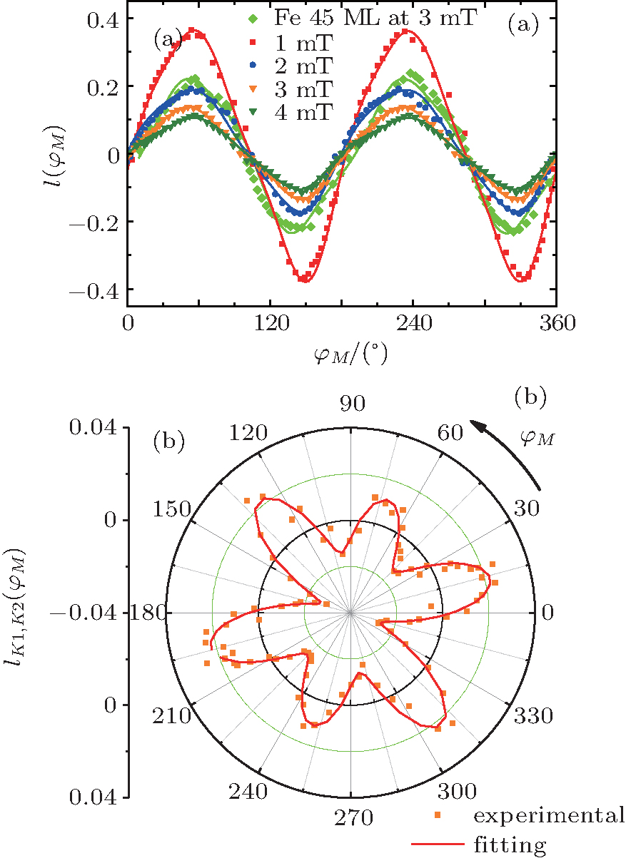


 , He Wei, Zhang Xiang-Qun, Sun Da-Li, Du Hai-Feng, Wu Qiong, Ye Jun, Fang Ya-Peng, Liu Hao-Liang]