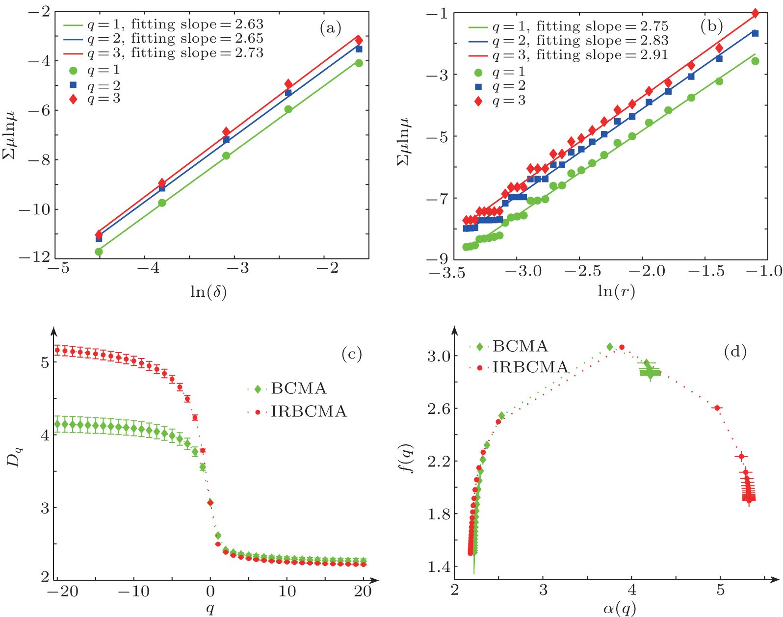
The multifractal analysis modified by Chhabra et al.^[18] is used for 3D BCMA and a typical MFS is shown in Fig. 1(a). Briefly, after dividing the 3D object into cubes with sizes δ × δ × δ , we assign a probability to each cube as 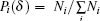, where N_i is a density at the i-th cube. To estimate the fluctuation of the density, the normalized q-th moment of the probability P_i(δ ) is defined as

where n is the number of the segmented cubes, and q can vary between − ∞ to + ∞ theoretically. Next, from the perspective of entropy, the singularity strength α (q) is given by

Meanwhile, the fractal dimension f(q) is given by

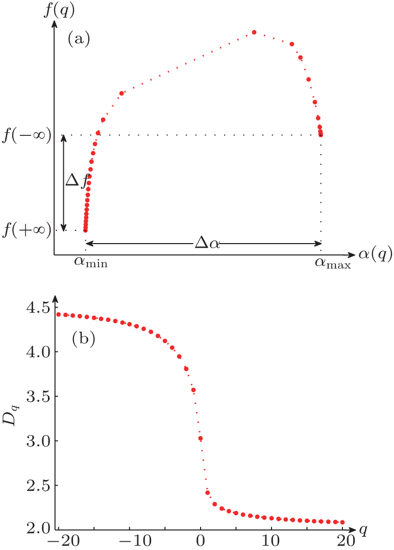
The plot of f(q) versus α (q) is called MFS, which is generally a hook-shaped curve, as illustrated in Fig. 1(a). In traditional BCMA, the “ power of 2” cube size (i.e., δ = 2ⁿ) is needed to divide the object for 3D MFS calculation in different scales.^[7] In this study, δ = 1, 2, 4, 8, 16 is used.

It should be noted that the value of q cannot be infinite in practice. In fact, if α (q) and f(q) tend to be constant, the maximum | q| can be deemed as the approximation limit of the endpoints. Following this idea, − 20 ≤ q ≤ 20 is used in this study. When q = − 20, the α (q) value is denoted as α _max, while the f(q) value is denoted as f(− ∞ ). Accordingly, the α _min and f(+ ∞ ) values are defined by α (q) and f(q) at q = 20, respectively. The positions of α _max, f(− ∞ ), α _min and f(+ ∞ ) are illustrated in Fig. 1(a).

In the traditional BCMA, only the divisions with δ = 2ⁿ are considered, which may omit some useful information beyond the restricted division size. Hence, we propose the 3D IRBCMA for calculation under arbitrary sizes.

Given a 3D object I with M × N × K voxels, for any ratio r(r ≥ 2, r ∈ Z⁺ ), we superpose a grid of blocks with m × n × k voxels, where m = ⌊ M/r⌋ , n = ⌊ N/r ⌋ , and k = ⌊ K/r ⌋ . Based on whether the values of M, N, and K could be exactly divided by r, there are eight situations to deal with.

Case 1M = mr, N = nr, and K = kr. The object is evenly partitioned into r × r × r blocks of m × n × k voxels.

Case 2M = mr, N = nr, and K > kr. The object is partitioned into r × r × (r + 1) blocks. Among these blocks, there are r × r × r blocks of m × n × k voxels and r × r × 1 blocks of m × n × (K − kr) voxels.

Case 3M = mr, N > nr, and K = kr. The object is partitioned into r × (r + 1) × r blocks. Among these blocks, there are r × r × r blocks of m × n × k voxels and r × 1 × r blocks of m × (N − nr) × k voxels.

Case 4M > mr, N = nr, and K = kr. The object is partitioned into (r + 1) × r × r blocks. Among these blocks, there are r × r × r blocks of m × n × k voxels and 1 × r × r blocks of (M − mr) × n × k voxels.

Case 5M = mr, N > nr, and K > kr. The object is partitioned into r × (r + 1) × (r + 1) blocks. Among these blocks, there are r × r × r blocks of m × n × k voxels, r × r × 1 blocks of m × n × (K − kr) voxels, r × 1 × r blocks of m × (N − nr) × k voxels, and r × 1 × 1 blocks of m × (N − nr) × (K − kr) voxels.

Case 6M > mr, N = nr, and K > kr. The object is partitioned into (r + 1) × r × (r + 1) blocks. Among these blocks, there are r × r × r blocks of m × n × k voxels, r × r × 1 blocks of m × n × (K − kr) voxels, 1 × r × r blocks of (M − mr) × n × k voxels, and 1 × r × 1 blocks of (M − mr)× n × (K − kr) voxels.

Case 7M > mr, N > nr, and K = kr. The object is partitioned into (r + 1) × (r + 1) × r blocks. Among these blocks, there are r × r × r blocks of m × n × k voxels, r × 1 × r blocks of m × (N − nr) × k voxels, 1 × r × r blocks of (M − mr) × n × k voxels, and 1 × 1 × r blocks of (M − mr)× (N − nr) × k voxels.

Case 8M > mr, N > nr, and K > kr. The object is partitioned into (r + 1) × (r + 1) × (r + 1) blocks. Among these blocks, there are r × r × r blocks of m × n × k voxels, r × r × 1 blocks of m × n × (K − kr) voxels, r × 1 × r blocks of m × (N − nr) × k voxels, 1 × r × r blocks of (M − mr) × n × k voxels, r × 1 × 1 blocks of m × (N − nr) × (K − kr) voxels, 1 × r × 1 blocks of (M − mr) × n × (K − kr) voxels, 1 × 1 × r blocks of (M − mr) × (N − nr) × k voxels, and 1 × 1 × 1 blocks of (M − mr) × (N − nr) × (K − kr) voxels.

After partitioning the object, for a certain ratio r, we define the intensity value T(i, j, k) in the (i, j, k)-th block. In order to contain the volume tightly and accurately, we allow the intensity value to be real, rather than integer. In addition, instead of using the difference of the maximum and minimum values in one block like Eq. (8) in Ref. [17], we take the sum of values as the measure, which can reflect more properties in the block. Thus, the intensity value in the (i, j, k)-th block is calculated as

where V(i, j, k) is the volume of the (i, j, k)-th block. The value of V(i, j, k) is equal to m × n × k for most blocks, but smaller for the remainder blocks along the object’ s borders. Next, similar to the BCMA in Section 2.1, the probability in the (i, j, k)-th block is measured by

The normalized q-th moment of the probability density is

Afterwards, as derived in Ref. [18], the singularity strength is then given by

and the fractal dimension can be calculated by

Generally, two strategies are commonly used for verifying multifractal characteristics in the box-counting method. In Ref. [18], different slopes from linearly fitting of ∑ μ lnμ with respect to lnL for different q values (usually q = 1, 2, 3) has been used as a simple and effective way to detect multifractal characteristics. In the BCMA case (see Fig. 3(a)), it refers to ∑ μ _i(q, δ ) ln μ _i(q, δ ) with respect to ln δ , while ∑ μ _q(i, j, k) ln μ _q (i, j, k) with respect to ln r is referred in the IRBCMA case (see Fig. 3(b)). Moreover, the “ generalized dimensions” , D_q, which correspond to scaling exponents for the q-th moments of the measure, can be achieved by

For an object with significant multifractal characteristics, the plot of D_q versus q is generally sigmoidal and decreasing.^[19] A typical illustration is shown in Fig. 1(b).

Fig. 1.

	Figure Option ViewDownloadNew Window
	Fig. 1. (a) Illustration of the typical MFS and the extracted features; (b) illustration of verifying multifractal characteristics.

According to the principle described in Ref. [20], the number of pixels covered by a particular grid block should be no less than the maximum number of the boxes in that block. Similar to this idea, the box size in the 3D IRBCMA method should meet the criteria of m × n × k = M/r × N/r × K/r ≥ r, which means . Meanwhile, m, n, and k should be large enough to form blocks, thus m = M/r ≥ 1, n = N/r ≥ 1, and k = K/r ≥ 1, i.e., r ≤ M, r ≤ N, and r ≤ K. We hereby obtain the upper limit of the box size . Moreover, to avoid only one block in the entire volume, r ≥ 2 should be satisfied. In practice, the lower bound should be adjusted according to the actual volume. Because the white matter only accounts for a small part in the whole brain volume, the closed range of 6 ≤ r ≤ Q is the reasonable box size used in this study.

For both BCMA and IRBCMA, two canonical features, Δ α and Δ f, are selected to capture the multifractal properties of white matter structure, which are shown in Fig. 1(a) as illustration.

The feature Δ α = α _max − α _min represents the width of the MFS, which can detect the degree of multifractality of the object. In the multifractal formalism, ^{[9, 18]} the distribution probability in the m-th box can be measured by P_m(r) ∝ (1/r)^{α _m}, where r (usually 0 < 1/r < 1) is the integer ratio forming the block size and α _m is the singularity strength of the probability subset. Obviously, P_m(r) increases with decreasing α _m at a fixed r. The value α _max is related to the minimum probability measure via P_min ∝ (1/r)^{α _max}, which corresponds to the smallest intensity values at scale 1/r. In contrast, α _min, measured via P_max ∝ L^{α _min}, corresponds to the largest intensity values at scale 1/r. The Δ α can thus be used to describe the range of the probability measures with P_max/P_min ∝ r^{Δ α} . The greater the Δ α value is, the wider the intensity distribution, the richer the structure, and the stronger the degree of multifractality in the object.

The feature Δ f = f(+ ∞ ) − f(− ∞ ) represents the difference of fractal dimension. In the formalism of Refs. [9] and [18], f(+ ∞ ) reflects the fractal dimension of the subset of the maximum probability with N_Pmax = N_{α min} ∝ (1/r)^{− f(+ ∞ )}, indicating the number of the largest intensity values, while f(− ∞ ) reflects the number of the smallest intensity values. Hence, the Δ f value can describe the ratio between the largest and the smallest intensity regions of the object: N_Pmax/N_Pmin ∝ (1/L)^{Δ f}.

MRI data used in this study were downloaded from the ADNI database. The ADNI was launched in 2003 by the National Institute on Aging (NIA), the National Institute of Biomedical Imaging and Bioengineering (NIBIB), the Food and Drug Administration (FDA), private pharmaceutical companies, and non-profit organizations as a $ 60 million, 5-year public private partnership. The primary goal of ADNI has been to test whether the combination of serial MRI, PET, other biological markers, and clinical and neuropsychological assessment can measure the progression of MCI and early AD. Determination of sensitive and specific markers of very early AD progression is intended to aid researchers and clinicians to develop new treatments and monitor their effectiveness, as well as lessen the time and cost of clinical trials. The principal investigator of this initiative is Michael W. Weiner, MD, VA Medical Center and University of California, San Francisco. The ADNI is the result of efforts of many co-investigators from a broad range of academic institutions and private corporations. The study subjects were recruited from over 50 sites across the US and Canada. They gave the written informed consent at the time of enrolment for imaging and genetic sample collection and completed the questionnaires approved by the Institutional Review Board (IRB) of each participating site.

Fig. 2.

	Figure Option ViewDownloadNew Window
	Fig. 2. Diagram of the preprocessing steps. Images are shown in 2D axial views.

Thirty-eight normal elderly controls (NC) (mean± SD: (77.2± 6.5) years) and twenty-five patients with early AD (mean± SD: (73.7± 7.6) years) were included. Among the subjects, twenty-eight NC and eleven early AD subjects were recorded with mini-mental state examination (MMSE) scores, which are extensively used to measure cognitive impairment and the dementia degree. The lower MMSE score is related to more severe cognitive impairment or dementia of the subject.^[21] The sagittal 3D T1-weighted magnetization prepared rapid gradient echo (MPRAGE) images with a resolution of 1 × 1 × 1.2 mm³ were acquired (TR = 6.8 ms; TE = 3.16 ms; flip angle is 9° ; thickness is 1.2 mm; matrix is 256 × 256).

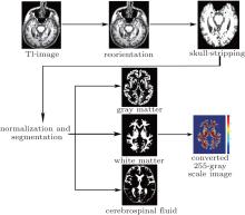
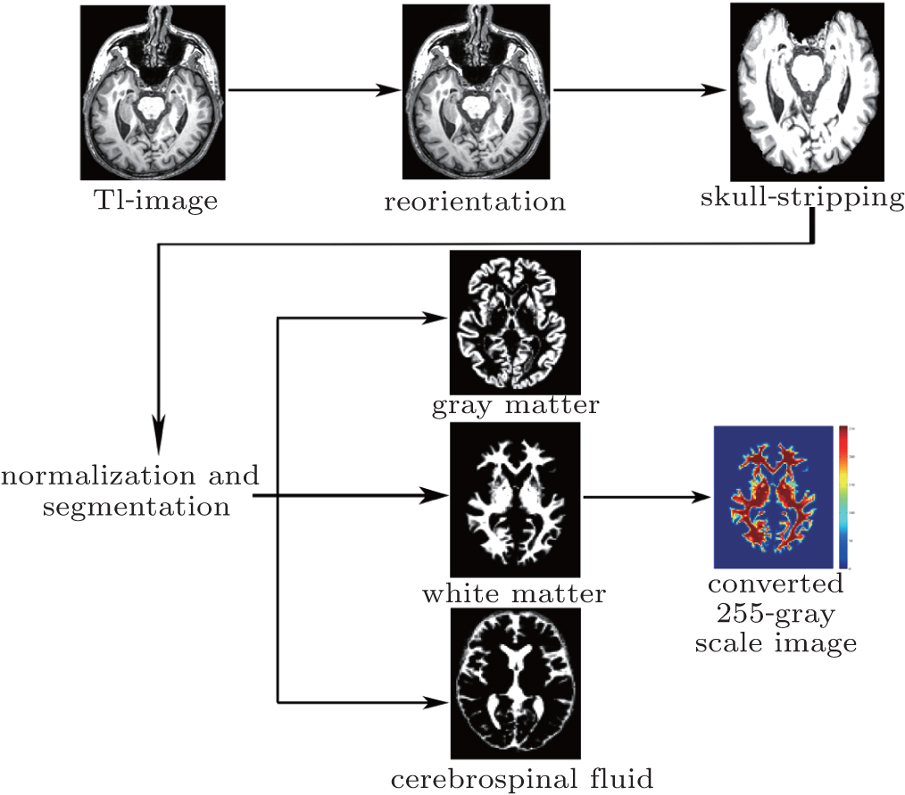
The standard preprocessing is shown in Fig. 2, which is performed using SPM8. The steps include manual reorientation, skull-stripping, spatial normalization to the MNI space, and segmentation into gray matter, white matter, and cerebrospinal fluid by employing diffeomorphic anatomical registration using the exponentiated liealgebra (DARTEL) method.^[22] Considering that the multifractal analysis evaluates the fluctuation of the objects, the MRI signal intensities were normalized and converted into 255-gray scale values to exclude the adverse effect of possible different intensity ranges among subjects. After preprocessing, the automatically segmented white matter was used for the further multifractal analysis.

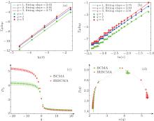
In this study, based on the preprocessed 3D MRI volumes of white matter, we firstly verified their multifractal characteristics by plotting the three fitted lines of ∑ μ lnμ with respect to lnL for q = 1, 2, 3 and the curves of D_q versus q for both BCMA and IRBCMA. The typical illustrations are shown in Fig. 3(a)– 3(c). Indeed for all subjects, the slopes of the three fitted lines for q = 1, 2, 3 are different and the D_q versus q curves tend to be sigmoidal and decreasing, which demonstrate that the 3D white matter volumes can be characterized by multifractals.

Fig. 3.

Figure Option ViewDownloadNew Window

Fig. 3. Three fitted lines with (a) Σ μ i lnμ i versus lnδ for BCMA and (b) Σ μ i lnμ i versus lnr for the IRBCMA are plotted to verify multifractal characteristics. The dot (• ), square (◻ ), and diamond (◊ ) symbols correspond to q = 1, q = 2, and q = 3 cases, respectively. In each case, linear fitting is performed and shown with the solid line, and its slope value is given in the legends. The multifractal characteristics is again verified by another plot from the same subject. (c) A plot of Dq versus q with q ranging from − 20 to 20 for both BCMA (◊ ) and IRBCMA (• ). Each curve is represented as mean ± standard error from different divisions. (d) A typical MFS from the same subject for both BCMA (◊ ) and IRBCMA (• ). Each point is represented as mean ± standard error from different divisions.

In our experiment, the averaged results from different divisions are used for more accurate multifractal results. The mean ± standard error for both BCMA and IRBCMA on MFS are plotted in Fig. 3(d). Multifractal features, Δ α and Δ f, were extracted based on the MFS. For both BCMA and IRBCMA, the statistic test results for both NC and AD groups are shown in Table 1. It clearly shows significant differences between NC and AD groups (p < 0.05) for both BCMA and IRBCMA, which suggests that Δ α and Δ f from both methods can effectively distinguish the NC and AD groups on 3D white matter MRI structure.

Table 1.

Table 1.

Table 1. Results of multifractal features for NC and AD groups. Δ α Δ f BCMA IRBCMA BCMA IRBCMA NC 1.99± 0.01 3.15± 0.01 – 1.35± 0.06 – 0.40± 0.07 AD 1.98± 0.01 3.14± 0.01 – 1.39± 0.08 – 0.47± 0.08 p 0.0051 0.0075 0.0076 0.0023

Table 1. Results of multifractal features for NC and AD groups.

In the previous studies, ^{[7, 10, 11]} only Δ α was reported to be a suitable multifractal feature of heterogeneity and used for exploring the white matter structural changes on MRI. As the measure for detecting multifractal degree, Δ α has been demonstrated to be effective in our study again. From Table 1, the larger Δ α value in NC group indicates that the NC group has wider intensity distributions and stronger multifractal structures than the AD counterpart, which is in line with the previous report of the smaller Δ α observed in patients.^[11] In addition to Δ α , the feature Δ f was also found to be sensitive in distinguishing NC and AD groups, which may suggest Δ f can be an alternative feature on such study. The Δ f value can describe the ratio between the largest and the smallest intensity regions of the white matter volume. In Table 1, Δ f < 0 is found for both NC and AD groups, which results from the small percentage of the white matter volume in the whole brain and hence the smaller number of regions with large intensity. Moreover, the Δ f values in NC group are larger than those in AD group, which may imply that in the brains, the proportion of the white matter volume in NC is larger than that in AD group. In Ref. [6], Migliaccio et al. employed the voxel-based morphometric analysis on NC and AD groups, and they found white matter atrophy in AD group. Our finding is in line with this report.

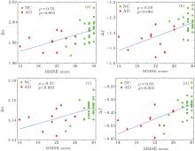
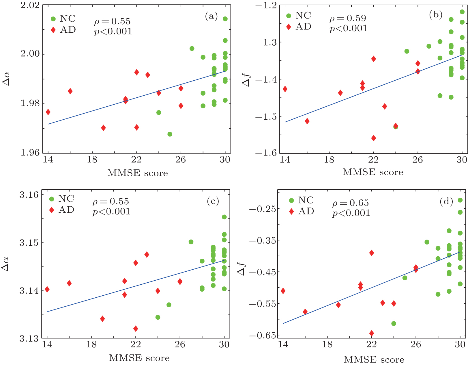
On the other hand, Pearson’ s correlation coefficient (ρ ) was used to test the association between the clinical MMSE scores and the multifractal features, as shown in Fig. 4. Strong positive correlations with statistical significance were found for both Δ α and Δ f with MMSE scores (ρ > 0.5 and p < 0.05). It is clearly suggested that the extracted multifractal features, Δ α and Δ f, are closely correlated with the clinical MMSE scores. Lower MMSE scores in AD subjects correspond to smaller Δ α and Δ f values, indicating the decline of complexity of white matter structure in the AD group.

Fig. 4.

Figure Option ViewDownloadNew Window

Fig. 4. Pearson’ s correlation coefficient ρ between the multifractal features and the clinical MMSE scores for (a) Δ α versus MMSE from BCMA; (b) Δ f versus MMSE from BCMA; (c) Δ α versus MMSE from IRBCMA; (d) Δ f versus MMSE from IRBCMA. The circle values (• ) are from NC subjects and the diamond values (◊ ) are from AD subjects. The solid line (— ) represents the correlation trend between the two values in the subfigures. p < 0.001 indicates the statistical significance for the Pearson’ s correlation coefficient.

It should be noted that both BCMA and IRBCMA were employed in this study. The traditional BCMA in the 2D case has been successfully applied for white matter structural changes on MRI.^{[7, 10, 11]} In this study, we extended it into the 3D case and obtained satisfactory results. However, BCMA is restricted to be calculated only on box size with 2ⁿ, which may neglect some useful information. Hence, we proposed the modified IRBCMA algorithm, which can relax the division to arbitrary box size. Our work was underpinned by the intuition that, the IRBCMA method can count boxes more accurately by capturing comprehensive information from arbitrary division. This is supported by the finding of the stronger correlation between Δ f and MMSE (ρ = 0.65, p < 0.05) by the IRBCMA compared with that obtained by BCMA (ρ = 0.59, p < 0.05), as shown in Figs. 4(b) and 4(d). Therefore, it may suggest that IRBCMA can be an alternative and more accurate algorithm for 3D volume analysis.