Wang Sheng-Hao, Margie P. Olbinado, Atsushi Momose, Hua-Jie Han, Hu Ren-Fang, Wang Zhi-Li, Gao Kun, Zhang Kai, Zhu Pei-Ping, Wu Zi-Yu. Experimental research on the feature of an x-ray Talbot–Lau interferometer versus tube accelerating voltage* . Chinese Physics B, 2015, 24(6): 068703
Permissions
Experimental research on the feature of an x-ray Talbot–Lau interferometer versus tube accelerating voltage*
Wang Sheng-Haoa)†, Margie P. Olbinadob), Atsushi Momoseb), Hua-Jie Hana), Hu Ren-Fanga), Wang Zhi-Lia), Gao Kuna), Zhang Kaic), Zhu Pei-Pingc), Wu Zi-Yua),c)‡
National Synchrotron Radiation Laboratory, University of Science and Technology of China, Hefei 230027, China
Institute of Multidisciplinary Research for Advanced Materials, Tohoku University, 2-1-1 Katahira, Aoba-ku, Sendai, Miyagi 980-8577, Japan
Institute of High Energy Physics, Chinese Academy of Sciences, Beijing 100049, China
*Project supported by the Major State Basic Research Development Program of China (Grant No. 2012CB825800), the Science Fund for Creative Research Groups, China (Grant No. 11321503), the National Natural Science Foundation of China (Grant Nos. 11179004, 10979055, 11205189, and 11205157), and the Japan–Asia Youth Exchange Program in Science (SAKURA Exchange Program in Science) Administered by the Japan Science and Technology Agency.
Abstract
X-ray Talbot–Lau interferometer has been used most widely to perform x-ray phase-contrast imaging with a conventional low-brilliance x-ray source, and it yields high-sensitivity phase and dark-field images of samples producing low absorption contrast, thus bearing tremendous potential for future clinical diagnosis. In this work, by changing the accelerating voltage of the x-ray tube from 35 kV to 45 kV, x-ray phase-contrast imaging of a test sample is performed at each integer value of the accelerating voltage to investigate the characteristic of an x-ray Talbot–Lau interferometer (located in the Institute of Multidisciplinary Research for Advanced Materials, Tohoku University, Japan) versus tube voltage. Experimental results and data analysis show that within a range this x-ray Talbot–Lau interferometer is not sensitive to the accelerating voltage of the tube with a constant fringe visibility of ∼ 44%. This x-ray Talbot–Lau interferometer research demonstrates the feasibility of a new dual energy phase-contrast x-ray imaging strategy and the possibility to collect a refraction spectrum.
X-ray phase-contrast imaging, which uses phase shift as the imaging signal, may provide a remarkably improved contrast over conventional absorption-based imaging for weakly absorbing samples, such as biological soft tissues and fibre composites.[1– 3] In the last 50 years, different x-ray phase-contrast imaging methods have been introduced. They can be classified as crystal interferometer, [4– 6] free-space propagation, [7, 8] diffraction enhanced imaging, [9, 10] and grating interferometer techniques.[11, 12] Although many experimental researches were performed with these techniques, at present none of them has been widely used in medical or industrial areas, where the use of a laboratory x-ray source and a large field of view are typically required. In 2006, Pfeiffer et al.[13] first developed and demonstrated a Talbot– Lau interferometer in the hard x-ray region with a conventional low-brilliance x-ray source. The experiment has been considered as a breakthrough in x-ray phase-contrast imaging, because it showed that phase-contrast x-ray imaging can be successfully and efficiently performed with a conventional, low-brilliance x-ray source, actually solving the problems that impaired a wider use of phase-contrast in x-ray radiography and tomography. Recently, potential applications of the method in biomedical imaging have been considered.[14– 17]
From the theoretical point of view, with a giving phase grating, because phase shift and Talbot distance of the phase grating are directly related to the wavelength of the x-ray, the ideal fringe visibility condition of an x-ray Talbot– Lau interferometer is valid only for a single wavelength. Moreover, with an x-ray Talbot– Lau interferometer, the accelerating voltage of the x-ray tube is chosen such that the mean energy of the radiation spectrum emitted from the radiation source matches the designed energy of the phase grating. However, in a real experiment, for samples with different attenuation abilities, the accelerating voltage of the x-ray tube needs to be adjusted to optimize the image contrast.[18] In addition, a dual energy x-ray phase-contrast imaging is of great interest for identifying, discriminating, and quantifying the materials existing in soft tissues. The present dual energy phase-contrast x-ray imaging strategy based on a Talbot– Lau interferometer adopts two distinct energy spectra, whose mean energies respectively match different orders of the Talbot distance.[19] A drawback of this method is however the low fringe visibility at the high energy (∼ 10% ), so that for a certain Talbot distance it is meaningful to explore the possibility of a new dual energy approach by choosing two energy spectra around the designed energy of the phase grating. As a consequence, the characterization of an x-ray Talbot– Lau interferometer versus the acceleration voltage of the tube is of particular relevance.
In the following sections, we will present and discuss the characterization of the x-ray Talbot– Lau interferometer (located in the Institute of Multidisciplinary Research for Advanced Materials, Tohoku University, Japan) versus the accelerating voltage of the tube. At first, the experimental setup, the image acquisition, and the data post-processing will be introduced. Then, we will present x-ray imaging results of a test sample and the curve of fringe visibility versus the accelerating voltage, and will discuss the calculations of δ (the decrement of the real part of the complex refractive index) and μ (the linear attenuation coefficient) of the test sample by numerical fitting for the different relations of acquisition versus voltage. The values of standard deviation σ of absorption, refraction, and visibility contrast image versus tube voltage will be also analyzed. Finally, we will discuss experimental data and present new potential application of this instrument.
2. Materials and methods
2.1. Experimental setup and working principle
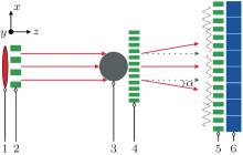
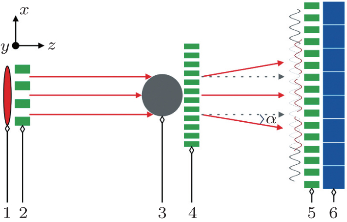
Grating-based x-ray phase-contrast imaging is carried out with an x-ray Talbot– Lau interferometer located at the Institute of Multidisciplinary Research for Advanced Materials at the Tohoku University, Japan. Figure 1 shows the layout of the x-ray interferometer. It is composed mainly of an x-ray tube, an x-ray detector, and three micro-structured gratings, which are assembled on multi-dimensional motorized optical stages. The x-ray radiation source is a tungsten rotating anode. The source grating G0 (period 22.7 μ m, Au height 70 μ m, size 20 mm× 20 mm) is located at about 80 mm from the emission point inside the x-ray source, the beam splitter grating G1 (period 4.36 μ m, Au height 2.43 μ m, size 50 mm× 50 mm) which induces a phase shift of π /2 at ∼ 27 keV, is placed 106.9 cm from G0 behind the gantry axis while the sample is set to be opposite and close to G1. The analyzer grating G2 (period 5.4 μ m, Au height 65 μ m, size 50 mm× 50 mm) is located at ∼ 10 mm in front of the detector while the distance between G1 and G2 is 25.6 cm. The x-ray detector is a combination of a scintillator and a CCD camera connected via a fiber coupling charge coupled device. The pixel size is 18 μ m× 18 μ m and the effective receiving area is 68.4 mm× 68.4 mm.
As illustrated in Fig. 1, the working principle of this Talbot– Lau interferometer can be briefly described as follows: the source grating G0, an absorbing mask with transmitting slits, placed close to the x-ray tube anode, creates an array of lines sources. Each line source is sufficiently small to prepare the required transverse coherence at the second grating (G1) that is coherently illuminated. In this way a self-image of G1 is formed in the plane of the grating G2 by the Talbot effect.[20] The images coming from all line sources look identical but they are shifted by multiples of the grating constant and therefore overlap in spite of their lack of mutual coherence. Moreover a Moire fringe is observed due to the superposition of the self-image and the G2 pattern in the plane of the x-ray detector. The differential phase-contrast image information process essentially relies on the fact that the sample placed in the x-ray beam path causes slight refraction of the beam transmitted through the object. The fundamental idea of differential phase-contrast imaging depends on locally detecting these angular deviations, the angular α is proportional to the local gradient of the object’ s phase shift, and can be quantified as
where Φ (x, y) is the phase shift of the wave front, and λ represents the wavelength of the radiation. Determination of the refraction angle can be achieved by combining the Moire fringe and phase-stepping technique, [21] a typical wave front measurement strategy which contains a set of images taken at different positions of the grating G2. When G2 scans along the transverse direction, the intensity measured in each pixel in the detector plane oscillates as a function of the grating position. From the Fourier analysis of the intensity signal of each pixel and looking at the shift curve of these oscillations, the conventional transmissions, refractions, and scattering signals of the samples as defined by Pfeiffer et al.[22] can be simultaneously retrieved.[12, 22]
Fig. 1. Layout of the x-ray Talbot– Lau interferometer. 1: the x-ray source; 2: source grating (G0); 3: sample; 4: beam splitter grating (G1); 5: analyzer grating (G2); 6: the x-ray detector.
2.2. Image acquisition and data post-processing
The sample we used is a PMMA cylinder with a diameter of 5 mm and a length of ∼ 100 mm. During the experiment, the x-ray generator operates with a tube current of 45 mA. After finely aligning the three gratings and the sample stage, the voltage is tuned to 35 kV. Five steps are adopted during the phase stepping scan, and for each step, 20 s is taken to collect a raw image. For measuring the background of the interferometer, the same phase stepping scan is performed after removing the PMMA cylinder. In the next step, we increase the tube voltage in steps of 1 kV up to 45 kV. At each step the same experimental procedure is adopted to carry out the phase-contrast x-ray imaging of the PMMA cylinder.
Regarding data post-processing, absorption image A (m, n), refraction image α (m, n), and the normalized visibility contrast signal V (m, n) of the sample are retrieved by a LabVIEW-based package using the NI Vision Development Module. The formulae we used are as follows:
where N is the number of steps during the phase stepping scan in one period of G2, (m, n) and (m, n) are the gray values of the pixel (m, n) at the k-th step of the scan with and without sample, respectively, p2 is the period of grating G2, and d is the distance between gratings G1 and G2.
3. Experimental results and data analysis
3.1. X-ray imaging results and the curve of visibility versus accelerating voltage
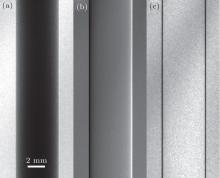
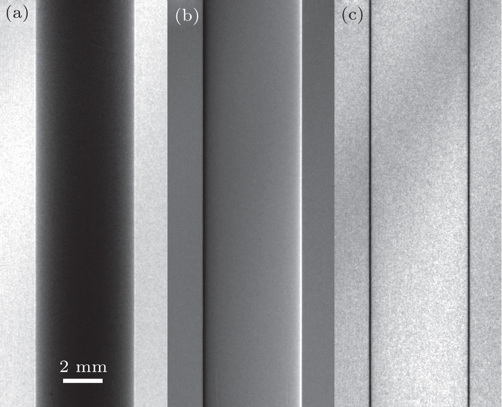
Figure 2 shows x-ray imaging results of the PMMA cylinder. Raw images are collected while the x-ray tube operates at an accelerating voltage of 35 kV. Figure 2(a) shows the conventional absorption image, while figure 2(b) displays the differential phase contrast signal, and figure 2(c) is the normalized visibility contrast image. All images are displayed with a linear gray scale and are windowed for optimized appearance. Here we should point out that no visual difference appears between the x-ray images obtained at the accelerating voltage of 35 kV and those collected at other voltages.
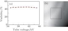
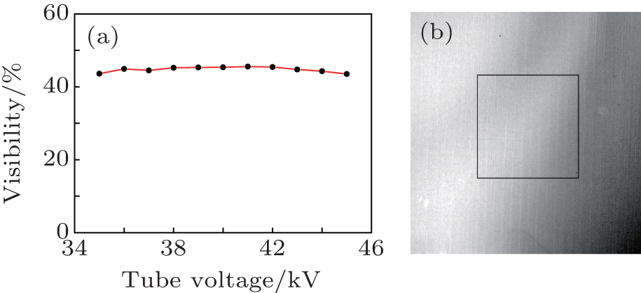
The fringe visibility of the x-ray Talbot– Lau interferometer for each value of the voltage is obtained by computing the visibility image without the sample in the beam path. The curve of the visibility versus the accelerating voltage of the tube is shown in Fig. 3(a), while displayed in Fig. 3(b) is the visibility image of the Talbot– Lau interferometer at 35 kV. The mean value in the black rectangle (800 pixels× 800 pixels) shown in Fig. 3(b) can be regarded as the visibility when plotting the curve in Fig. 3(a). We should underline here that the vertical stripes in the visibility image as demonstrated in Fig. 3(b) reveal some interesting details of the background of the Talbot– Lau interferometer, while Au grids of the grating in the beam path act as an important medium for visibility signal retrieval, both the still existing photoresists and the silicon wafers of the background can be regarded as the sample under analysis.
Fig. 2. The x-ray imaging results of the PMMA cylinder obtained at an accelerating voltage of 35 kV, showing (a) conventional absorption image, (b) refraction signal, and (c) normalized visibility image. All the images are windowed for optimized appearance with a linear gray scale.
Fig. 3. (a) Curve of fringe visibility versus the accelerating voltage of the tube; (b) visibility image without the sample at 35 kV. The mean value in the black rectangle (800 pixels× 800 pixels) is regarded as the fringe visibility when plotting the curve in panel (a).
3.2. δ , μ of PMMA and Vs/Vb versus accelerating voltage
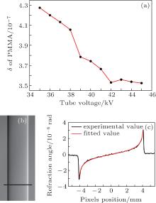
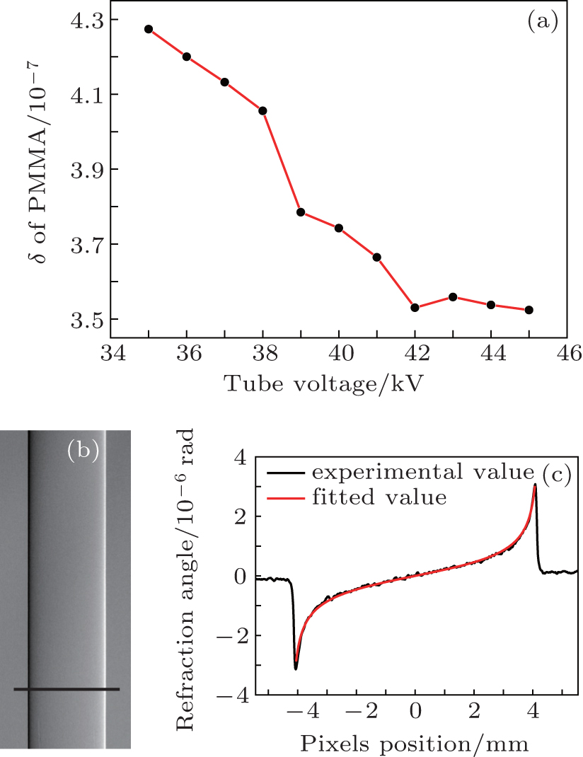
The curve of δ (the decrement of the real part of the complex refractive index of PMMA) versus accelerating voltage is displayed in Fig. 4(a), while figures 4(b) and 4(c) show the calculation results of δ by a numerical fit at 35 kV. The black curve in Fig. 4(c) is the refraction signal of the cross section chosen as shown in Fig. 4(b). Here 30 rows are chosen to minimize the noise of the refraction signal, and the red line in Fig. 4(c) is the best fit curve when δ equals 4.27399× 10− 7. The formula used for the fit is
where R is the radius of the PMMA cylinder, x is the variable, and θ is the refraction angle. The fit is performed with the Levenberg– Marquardt algorithm.[23]
Fig. 4. (a) δ of the PMMA versus accelerating voltage; (b) and (c) the computing process of δ at 35 kV. The black curve in panel (c) is the refraction signal of the cross section chosen as in panel (b) and the red line in panel (c) is the best fit curve when δ is 4.27399× 10− 7.
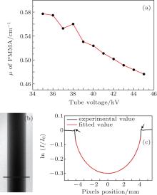
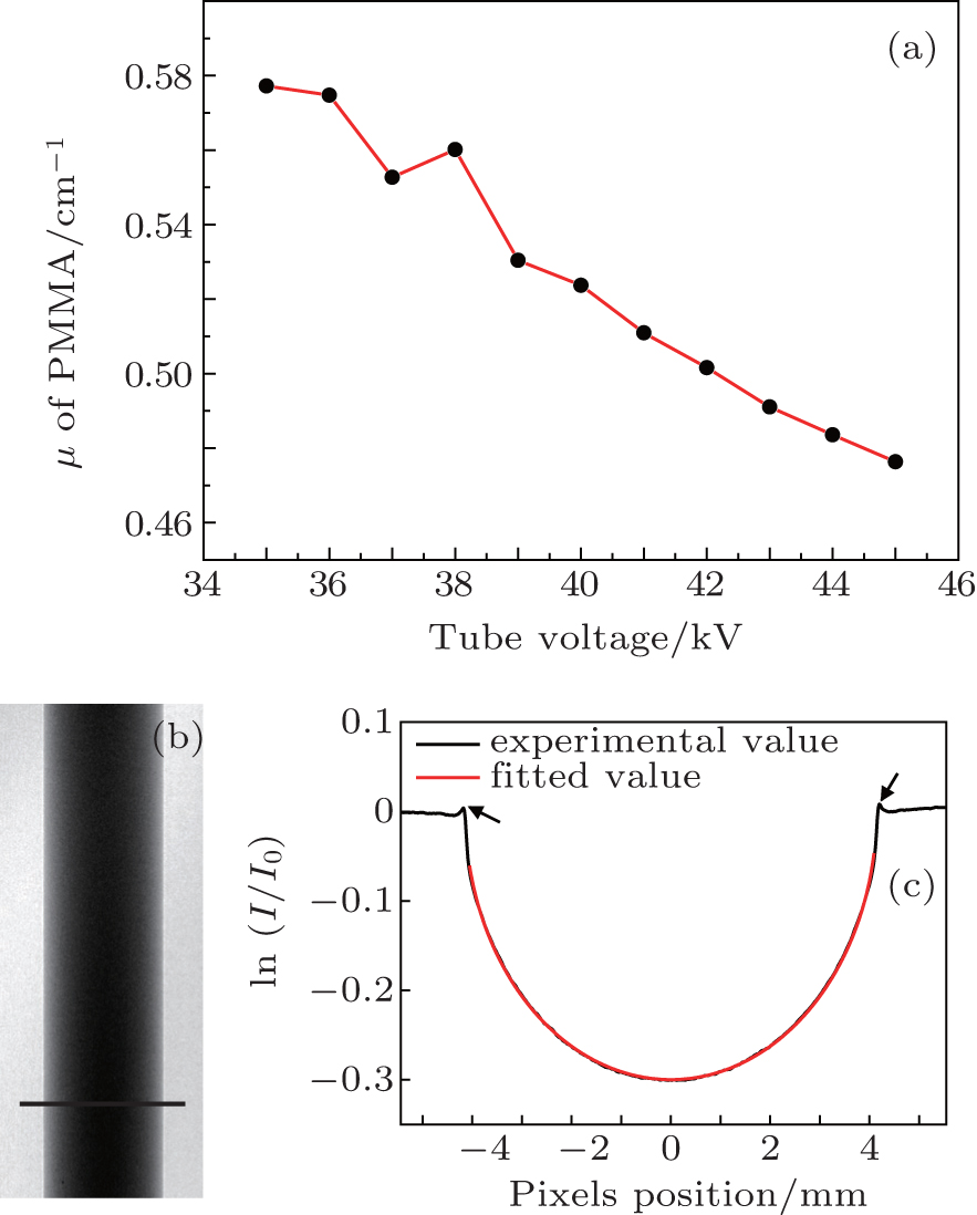
Fig. 5. (a) μ of PMMA versus accelerating voltage, (b) and (c) the computing process of μ at 35 kV. The black curve in panel (c) is the absorption projection value of the section profile chosen as shown in panel (b), while the red line in panel (c) is the best fit curve when μ is 0.57724 cm− 1. The two small peaks indicated by the black arrows in panel (c) point out the edge enhanced phenomenon in the retrieved absorption image.
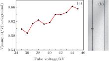
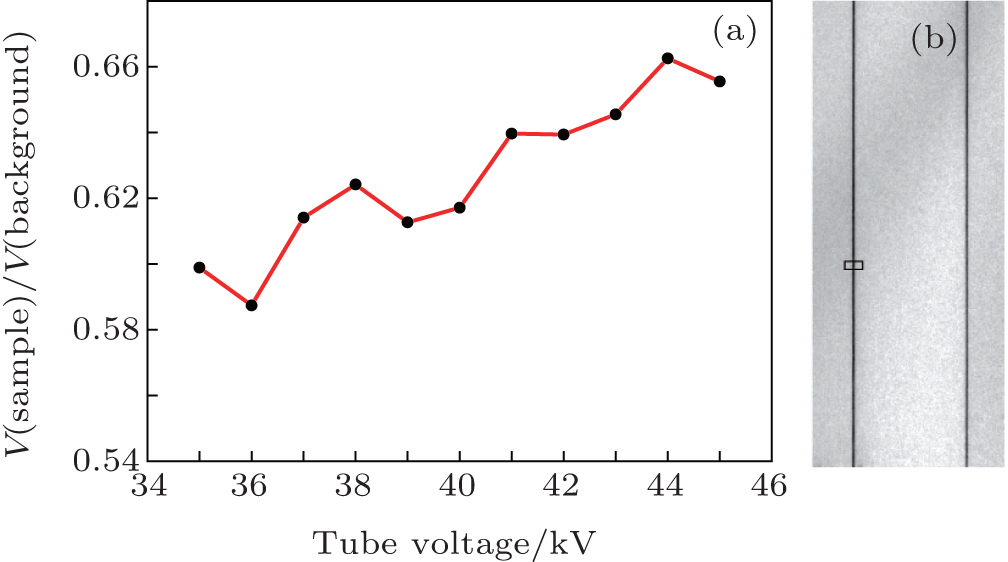
Fig. 6. (a) Curve Vs/Vb versus accelerating voltage, and (b) the visibility image of Vs/Vb obtained at the voltage of 35 kV, pixels of the black line located inside the rectangular (2 pixels× 10 = 20 pixels) are averaged to generate the curve.
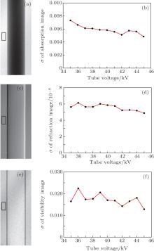
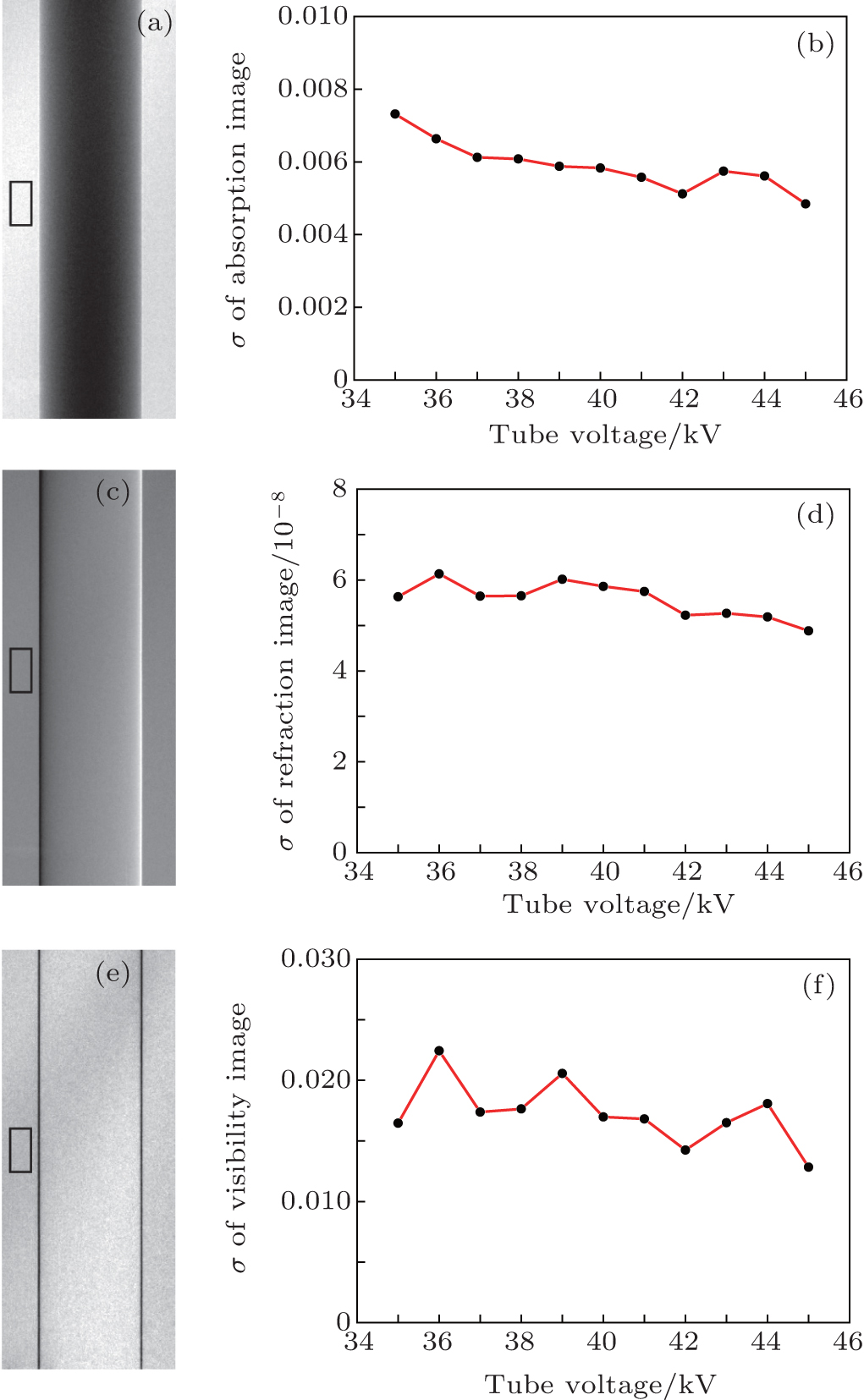
Fig. 7. (a) Absorption image, (c) refraction signal, and (e) normalized visibility image, at a voltage of 35 kV; values of σ of (b) absorption, (d) refraction, and (f) visibility images versus accelerating voltage. Pixels in the rectangle (30 pixels × 100 = 3000 pixels) in panels (a), (c), and (e) are used to compute the values of σ of the absorption/refraction/visibility images, respectively.
Similarly, the curve of μ , the computed linear attenuation coefficient of the PMMA versus accelerating voltage is shown in Fig. 5. For the variance of the fit formula that generates δ , we use the fitting equation
where I and I0 are the gray values of the x-ray images obtained with and without sample, respectively.
The values of visibility signal that is defined as Vs/Vb (where Vs and Vb represent the visibility images of the Talbot– Lau interferometer with and without sample, respectively)[22] at each voltage value are calculated and the curve of Vs/Vb versus accelerating voltage is shown in Fig. 6(a). Figure 6(b) shows the image of Vs/Vb at the voltage of 35 kV. All pixels of the black line located inside the rectangle (2 pixels× 10 = 20 pixels) are averaged to generate the curve.
3.3. Values of σ of absorption, refraction, and visibility signals versus accelerating voltage
The values of standard deviation σ of absorption, refraction, and visibility images versus accelerating voltage are shown in Figs. 7(b), 7(d), and 7(e), respectively. Pixels in the black rectangle (30 pixels× 100 = 3000 pixels) shown in Figs. 7(a), 7(c), and 7(e) are used to compute the values of σ for all images.
4. Discussion
In Fig. 2 we compare the three imaging signals of the PMMA cylinder. Here we should point out that the retrieved absorption image shown in Fig. 2(a) is a pseudo-absorption image, which is identical to the transmission image that is obtained if the Talbot– Lau interferometer is not inserted along the beam path. It contains the projected absorption coefficient and the edge-enhancing Fresnel diffraction contrast.[24, 25] We can obtain the evidence in Fig. 2(a) that the edge of the PMMA cylinder is slightly brighter than other parts of the background, and also in Fig. 5(c), the retrieved absorption signal of the cross section, we can detect a small peak appearing at both edges of the cylinder as indicated by the black arrows.
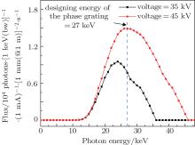
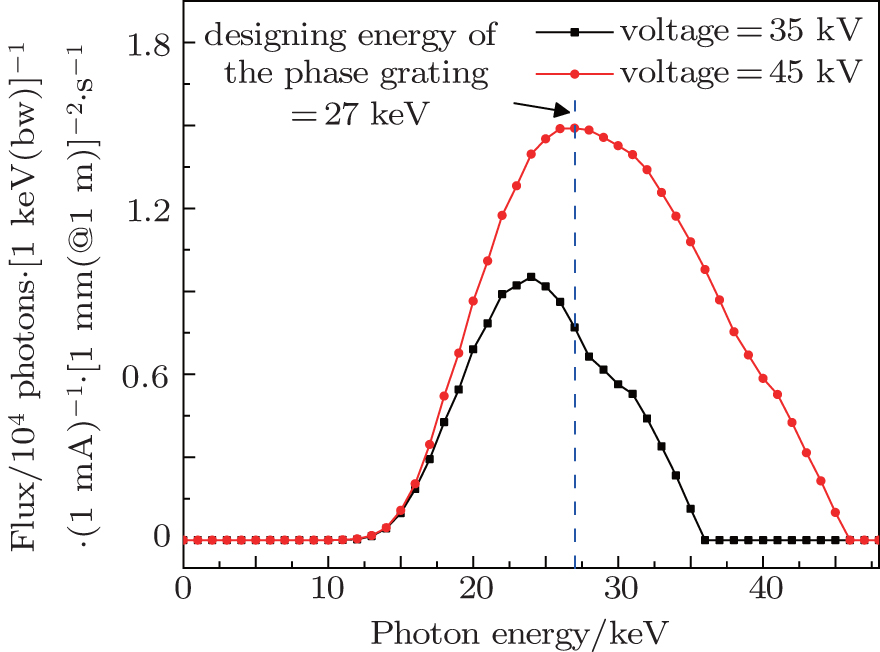
Fig. 8. Black and red lines show the emission spectra of the x-ray tube at the accelerating voltage of 35 kV and 45 kV, respectively. The blue dashed line indicates the designed energy of the phase grating (27 keV).
As shown in Fig. 3(a), the fringe visibility slowly increases from 35 kV to 41 kV and after that it starts to decrease. The behavior can be explained because the phase grating of the x-ray Talbot– Lau interferometer is designed for an energy of 27 keV, which is indicated in Fig. 8 with the blue dashed line. The black and the red lines in Fig. 8 show the emission spectra of the x-ray tube for accelerating voltages 35 kV and 45 kV respectively, while the spectra at voltages from 36 to 44 kV are not shown (the emission spectra of the x-ray tube is calculated by the XOP 2.1 software[26]). The optimal fringe visibility is achieved when the mean energy of the emission spectrum of the x-ray tube well matches the design energy, and when the mean energy of the emitted spectrum starts to deviate from the design energy of the phase grating, the visibility worsens. However, what is also clearly seen from the data is that the fringe visibility of this x-ray Talbot– Lau interferometer varies smoothly and still remains at a relatively high level in a voltage range of 35 kV– 45 kV. The worst visibility we measured in the experiment is 43% at 45 kV. Since the fringe visibility is a key parameter of the Talbot– Lau interferometer for both refraction and scattering signal retrieval, [27– 30] we may claim that this x-ray Talbot– Lau interferometer can be well utilized to perform the experiments in experimental layouts where the tube accelerating voltage needs to be changed, and at the same time also a high fringe visibility is required. As an example: (i) when samples with different attenuation properties are to be investigated, the accelerating voltage of the x-ray tube needs to be adjusted to optimize the image contrast.[18] (ii) In dual energy x-ray phase-contrast imaging, both a low-energy and a high-energy spectrum are separately measured by changing the accelerating voltage of the x-ray tube. In the present dual energy x-ray phase contrast imaging strategy based on a Talbot– Lau interferometer, the two energy spectra are chosen such that the mean energies of the two spectra match different orders of the Talbot distance.[19] Actually, the main drawback of this method is that the fringe visibility at the high energy is too low (10% ). On the contrary, changing the tube accelerating voltage around the designed optimal value, we hope a new dual energy x-ray phase-contrast imaging strategy can be implemented with a fringe visibility producing a higher image quality, i.e., by collecting two energy spectra around the designed energy of the phase grating, even though the tube voltage range is limited to a certain range. In our experiment with a PMMA cylinder, dual energy x-ray imaging phase-contrast data are obtained with the values of δ equaling 4.27× 10− 7 at 35 kV and 3.52× 10− 7 at 45 kV, while the values of μ being 0.57724 cm− 1 at 35 kV and 0.47634 cm− 1 at 45 kV. (iii) Finally, in a rough refraction spectrum measurement as shown in Figs. 4(a) and 5(a), δ and μ of the PMMA are measured with a conventional x-ray tube source in a voltage range of 35 kV– 45 kV. This measurement may find potential applications in elemental recognition and materials discrimination. As shown in Fig. 6(a) we find also that the visibility signal of the PMMA is related to the tube accelerating voltage. The potential use of this feature is similar to the other two signals.
Finally in the previous section, we calculated the values of standard deviation σ of the absorption, refraction, and visibility contrast signals and plotted the curves of σ versus tube accelerating voltage in Fig. 7. From the theoretical point of view the σ of the refraction signal retrieved from an x-ray Talbot– Lau interferometer is closely related to the fringe visibility, while those of absorption and scattering signals are not.[31] However, as shown in Figs. 7(b), 7(d), and 7(f), the values of σ for all signals slowly decrease while the tube accelerating voltage increases. The behavior can be explained by considering that the radiation emitted from the x-ray tube is roughly proportional to the second order of the accelerating voltage and the effect of the small change of the fringe visibility in a voltage range of 35 kV– 45 kV associated with the noise of the refraction image is negligible. Actually, the analysis of σ of the refraction signal versus accelerating voltage strongly supports the evidence that this x-ray Talbot– Lau interferometer is almost insensitive to the accelerating voltage in the range of 35 kV– 45 kV. As a consequence, based on the above discussion on the fringe visibility, this x-ray Talbot– Lau interferometer can be used to perform experiments where the accelerating voltage needs to be changed and also imaging quality needs to be guaranteed.
Finally, we should point out that this experimental research is limited to the x-ray Talbot– Lau interferometer located in Tohoku University. The extensive and comprehensive discussion about all features of an x-ray Talbot– Lau interferometer versus accelerating voltage, also with consideration of gratings imperfections and various mechanical design, will be more universal and is thus expected.
5. Conclusions
In this work, the characteristics of an x-ray Talbot– Lau interferometer versus accelerating voltage of the x-ray tube is investigated by using a test sample through changing the accelerating voltage of the radiation source. Experimental results and data analysis show that this x-ray Talbot– Lau interferometer is almost insensitive to the accelerating voltage in a range from 35 kV to 45 kV. This experimental research shows that a new dual energy phase-contrast x-ray imaging approach and rough refraction spectrum measurements within a certain range are feasible with this x-ray Talbot– Lau interferometer.
Acknowledgment
The authors are grateful to Murakami Gaku, Wataru Abe, Taiki Umemoto, and Kosuke Kato of the Institute of Multidisciplinary Research for Advanced Materials of the Tohoku University for their kind help while running the experiments, and also to Augusto Marcelli of the Istituto Nazionale di Fisica Nucleare-Laboratori Nazionali di Frascati for fruitful discussions.
ZanetteI, WeitkampT, LangS, LangerM, MohrJ, DavidC and BaruchelJ2011Phys. Status Solidi A2082526DOI:10.1002/pssa.201184276[Cited within:1][JCR: 1.463]
26
Del RíoM S, DejusR J and Dejus2004Synchrotron Radiation Instrumentation: Eighth International Conference on Synchrotron Radiation Instrumentation25–29 August, 2003San Francisco, California (USA)784[Cited within:1]
... [11,12] Although many experimental researches were performed with these techniques, at present none of them has been widely used in medical or industrial areas, where the use of a laboratory x-ray source and a large field of view are typically required ...
2
2003
1.067
0.0
... [11,12] Although many experimental researches were performed with these techniques, at present none of them has been widely used in medical or industrial areas, where the use of a laboratory x-ray source and a large field of view are typically required ...
... [12,22] ...
1
2006
19.352
0.0
... [13] first developed and demonstrated a Talbot#cod#x2013 ...
1
2011
2.701
0.0
... [14#cod#x2013 ...
1
2013
0.0
0.0
1
2013
1.407
0.0
1
2014
2.891
0.0
... 17] ...
2
1983
1.142
0.0
... [18] In addition, a dual energy x-ray phase-contrast imaging is of great interest for identifying, discriminating, and quantifying the materials existing in soft tissues ...
... [18] (ii) In dual energy x-ray phase-contrast imaging, both a low-energy and a high-energy spectrum are separately measured by changing the accelerating voltage of the x-ray tube ...
2
2010
0.71
0.0
... [19] A drawback of this method is however the low fringe visibility at the high energy (#cod#x0223C ...
... [19] Actually, the main drawback of this method is that the fringe visibility at the high energy is too low (10#cod#x00025 ...
1
1836
0.0
0.0
... [20] The images coming from all line sources look identical but they are shifted by multiples of the grating constant and therefore overlap in spite of their lack of mutual coherence ...
1
1974
0.0
0.0
... Determination of the refraction angle can be achieved by combining the Moire fringe and phase-stepping technique,[21] a typical wave front measurement strategy which contains a set of images taken at different positions of the grating G2 ...
3
2008
35.749
0.0
... [22] can be simultaneously retrieved ...
... [12,22] ...
... Lau interferometer with and without sample, respectively)[22] at each voltage value are calculated and the curve of Vs/Vb versus accelerating voltage is shown in Fig ...
1
1978
0.0
0.0
... [23] ...
1
2005
3.546
0.0
... [24,25] We can obtain the evidence in Fig ...
1
2011
1.463
0.0
... [24,25] We can obtain the evidence in Fig ...
1
2004
0.0
0.0
... 1 software[26]) ...
1
2008
3.546
0.0
... Lau interferometer for both refraction and scattering signal retrieval,[27#cod#x2013 ...
1
2010
1.367
0.0
1
2011
1.142
0.0
1
2014
1.016
1.691
... 30] we may claim that this x-ray Talbot#cod#x2013 ...
1
2010
0.0
0.0
... [31] However, as shown in Figs ...
Experimental research on the feature of an x-ray Talbot–Lau interferometer versus tube accelerating voltage*
[Wang Sheng-Haoa)†, Margie P. Olbinadob), Atsushi Momoseb), Hua-Jie Hana), Hu Ren-Fanga), Wang Zhi-Lia), Gao Kuna), Zhang Kaic), Zhu Pei-Pingc), Wu Zi-Yua),c)‡]


 , Margie P. Olbinado