


Reweighted ensemble dynamics simulations: Theory, improvement, and application*
[Gong Lin-Chena) , Zhou Xinb)†  , Ouyang Zhong-Can
a), c) ]
, Ouyang Zhong-Can|
|


†Corresponding author. E-mail: xzhou@ucas.ac.cn
*Project supported by the National Natural Science Foundation of China (Grant No. 11175250).
Based on multiple parallel short molecular dynamics simulation trajectories, we designed the reweighted ensemble dynamics (RED) method to more efficiently sample complex (biopolymer) systems, and to explore their hierarchical metastable states. Here we further present an improvement to depress statistical errors of the RED and we discuss a few keys in practical application of the RED, provide schemes on selection of basis functions, and determination of the free parameter in the RED. We illustrate the application of the improvements in two toy models and in the solvated alanine dipeptide. The results show the RED enables us to capture the topology of multiple-state transition networks, to detect the diffusion-like dynamical behavior in an entropy-dominated system, and to identify solvent effects in the solvated peptides. The illustrations serve as general applications of the RED in more complex biopolymer systems.
Exploring for the high-dimensional conformational space of complex molecular systems has long been the focus of computer simulation studies in recent years. Two challenges exist under this topic, i.e., how to thoroughly sample the conformational space, and how to understand the equilibrium and dynamic properties based on lots of simulation data in hand. Although standard Monte-Carlo (MC) and molecular-dynamics (MD) simulation methods have been widely applied and achieved great successes, for many complex systems, such as glassy systems, phase-transition systems, and solvated biopolymers, sufficient sampling is by no means an easy task. The rugged energy landscapes in the systems frequently trap simulation trajectories in a small conformational region, disallowing the thorough exploration of the whole conformational space within limited simulation time. Due to those, lots of various advanced simulation techniques, such as umbrella sampling, [1– 3] J-walk, [4] multicanonical ensembles, [5] simulated tempering, [6, 7] conformational flooding, [8] hyperdynamics, [9– 11] parallel tempering, [12, 13] Wang– Landau sampling[14] and its derivatives, [15, 16] meta-dynamics, [17] and multidimensional generalized-ensemble methods, [18] have been developed and applied to overcome the difficulties. New hardware[19] and parallel computational technique[20] were also designed to extend MD simulations to reach microsecond scale in protein systems. On the other hand, due to the growing power of massively distributed computation, the ensemble dynamics (ED), [21– 23] which independently runs multiple simulations in distributed computers, provides an alternative way for bridging the gap between simulation power and practical interest.
Besides efficiently sampling, proper analysis and understanding systems from the simulation data are also not a trivial task. The major purpose in data analyses, is to search for a coarse-grained description of the conformational space. In the traditional way, a few (usually only one or two) knowledge-based reaction coordinates (or order parameters) are first defined, then the equilibrium (and dynamic) properties of the system are achieved by mapping sampled configurations in the low-dimensional reaction-coordinate space. However, this method may suffer from the arbitrariness in the selection of reaction coordinates, and give an oversimplified description of the system.[24] Recently, a systematic metastable-state-network-based view brought prominent improvement.[25– 34] Due to being theoretically transparent and inclusive of nearly all the useful information, the network model has received much attention.
In a previous work, [35] we have proposed a method, which was previously denoted as the weighted ensemble dynamics, now renamed as the reweighted ensemble dynamics (RED), to enhance sampling and to form a metastable-state transition network.[36] The RED is following the spirit of ED, which generated multiple short simulation trajectories from dispersively-chosen initial conformations, then applies a network-based analysis to get equilibrium and dynamics properties from all of these trajectories. In the present paper, we further improve and validate the RED, including: (i) we present a scheme to select basis functions and judge their completeness; (ii) we discuss the unique free parameter in the RED; (iii) we provide an improvement to depress statistical errors. We illustrate the improved RED in a few different systems, give the topology structure of a multiple-state transition network, and predict the diffusion-like dynamical property in entropy-dominated systems. More importantly, we apply the RED to analyze the effects of different aspects (degrees of freedom, interactions, etc.) separately, such as the solvent effects in the solvated dipeptide.
The article is organized as follows. In Section 2, we briefly represent the main formula of the RED, then we discuss a few keys in the RED, such as selection of basis functions, the effects of unique parameters, and the improvement of statistical errors. In Section 3, we illustrate the application of the RED in two-dimensional multiple-well potentials and in solved dipeptides. A short conclusion is given in Section 4. The simulation and analysis details are presented in Appendix A.
In the RED, multiple MD (or MC) trajectories, {qi(t)}, i = 1, … , p, t ∈ [0, τ ], are independently generated from initial conformations, denoted as {qi(0) = qi0}, i = 1, … , p, under the same simulation condition, respectively. Each trajectory involves m conformations, {qi(t = jΔ ) = qi, j}, j = 0, … , m − 1, thus total m × p conformations are sampled. Here q is a simple notation of configurational coordinates. Δ ; is the time interval of the samples, and mΔ ; = τ . We denote the distribution of samples in a single trajectory as 

Usually, while τ is shorter than the equilibrium time of systems, a single trajectory does not reach the equilibrium, i.e., Pi(q) ≠ Peq(q), but we can use all of these trajectories to reproduce the equilibrium distribution,

where wi is the weight of the i-th trajectory, which is due to the deviation of the initial distribution from the equilibrium distribution. A possible selection of {wi} is,

Thus, we have a linear equation about {wi},

where

and ∑ jwj = p.
Due to the finite size of samples {qi, j}, equation (1) should be understood as

for any A(q), while 〈 A(q)〉 i is estimated as 

while 〈 … 〉 α is estimated by average in the corresponding conformation samples. By expanding on a complete set of conformational functions (named as basis functions) {Aμ (q)}, μ = 1, 2, … , we have,

Here gμ ν is the inverse of gμ ν ≡ 〈 Aμ (q) Aν (q)〉 init which is estimated by the average in the initial sample.
In practical application, instead of A(qi, 0) in estimation of Γ ij, we use the average of A(q) in a short t̃ -length initial segment of trajectory (the first m0 configurations with m0 ≪ m or t̃ ≪ τ ), i.e.,

then

Here {Â μ (q)} is the orthonormalized basis functions satisfying 〈 Â μ (q)Â ν (q)〉 init+ = δ μ ν with

Thus, equation (3) can be rewritten as

Here H ≡ GTG is the variance– covariance matrix of the trajectory-mapped vectors

where Gij ≡ Γ ij − δ ij with i = 1, … , p, and w = (w1, … , wp)T. Equation (6) is the main formula of the RED. The w corresponds to the ground state of matrix H whose number of degenerated ground states gives the number of disconnected metastable states under the timescale of the individual trajectory τ , the existence of a small fraction of transition trajectories among states can slightly split the ground state of H. More details are shown in our previous work.[35]
The selection of basis functions is a key in the practical application of RED. In our previous works, [35, 36] we briefly discussed the selection of basis functions, and used some triangle functions as basis functions like Fourier expansion. Here we more generally discuss the key point of the RED.
Although the expansion in the RED required a complete set of basis functions in principle, it is usually not necessary to include too many basis functions in practice. Usually, it is easy to choose the initial configurations so that its distribution Pinit+ (q) is already local equilibrium, thus only slow processes need to be reweighted by the RED. Therefore Ω (q) in the all-atomic q space can be replaced by Ω (x) = Peq(x)/[Pinit+ (x)] in a coarse-grained x space, where x represents the slow (coarse-grained) degrees of freedom, P(x) is the corresponding distribution function in the x space. For example, in proteins, if we disregard the first few nanoseconds of relaxation simulation and reset the zero point of time, it is safe to suppose only some slow degrees of freedom, such as torsion angles of backbone, positions of side-chain atomic groups, be x, thus only functions in the x space should be applied as basis functions. In many cases, systems might reach equilibrium within the τ time (length of individual trajectory) except for only a few collective variables, thus we even apply the RED in a low-dimensional space. In addition, we usually suppose there are many potential-energy basins (or super-basins) separated by high (free) energy barriers in the conformational space; each (super-)basin corresponds to a metastable state wherein a τ -length trajectory is sufficient to reach local equilibrium. Thus, Ω (x) looks like a step-like function, which is almost constant in each metastable state, variations only happening at boundaries between states. We approximately have

where Θ α (x) is character function of the α metastable state, which is unity if x is inside the state, zero otherwise. The set of character functions of states {Θ α (x)} provides a natural set of basis functions to expand Ω (x), thus the required number of basis functions is equal to the number of states. Since the boundaries of these states are unknown a priori, we usually use far more basis functions to linearly combine the step-like Ω (x) function. We may use some usual collective variables with clear physical meaning as basis functions. In biological macromolecules, dihedral angles and their analytical functions, pair distances between some key atomic groups, potential energy or its parts, solved area of proteins, radius of gyration, native contact number, number of hydrogen, etc., can be applied as basis functions. The variance– covariance matrix gμ ν will ensure the consistent consideration of different classes of basis functions, and provide the measure of their relative importance by the orthonormalization process. In addition, the number of independent basis functions is also limited by the finite size of init+ , thus more selected basis functions will be discarded after considering the matrix gμ ν , then do not significantly contribute to final results. Another possible scheme about the selection of basis functions is to use local functions in the conformational space. For example, for a set of sampled configurations, {xi}, i = 1, … , M, one may group them into some subsets by clustering algorithms based on their geometric similarity, and use the character functions of clusters as basis functions. Thus the number of basis functions is the number of clusters, ncl = M/m. Here M and m are the total number of sampled conformations and the (average) number of conformations in each cluster. The idea is actually already applied in the Markov State Model (MSM) to divide the whole conformational space into metastable states.[24, 30– 34] In this paper, we use physically meaningful collective variables as basis functions, the application of the sample-based discrete cluster functions will appear elsewhere.
The completeness of selected basis functions can be directly test-based on sampled configurations in the RED. For a set of basis functions {Aμ (x)}, we can estimate the difference between two samples (or the corresponding distributions), such as the initial distribution Pinit+ (x) and the equilibrium distribution Peq(x),

The definition gives a measurement about the similarity of samples, and can be generally applied to compare two samples. For example, we had used the formula to optimize coarse-grained models of the all-atomic water.[37] For assessing the completeness of basis functions in the expansion of Peq(x)/[Pinit+ (x)], a reasonable method is to check the convergence of 
To calculate 


Since the statistical errors exist due to the finite sample sizes, S2 would not strictly stop growing with the number of basis functions, it just increases slowly compared to the initial growing phase with increasing basis functions. Similarly, when a large error occurs, S2 may abnormally increase within the saturation region. We design a scheme to get rid of the statistically unreliable basis functions. We orthonormalize the functions {Aμ (x)}, leading to the explicitly identifiable value and error contribution from the orthonormalized basis functions to S2. In the present paper, we implement the Gram– Schmidt orthonormalization method to one-by-one derive out the set of orthonormalized basis functions {Â μ (x)}, thus 

Here, Err( ) denotes the statistical error of the quantity in brackets. For each orthonormalized basis function, Â μ , if Err(sμ ) is larger than | sμ | , i.e., the relative error of sμ is larger than 1.0, this basis function will not be selected in expansion. One-by-one selection will give out the final basis function set and the estimated error of the completeness measure S2.
The scheme introduced here provides us with the knowledge about how many basis functions are enough in the RED. After orthonormalization, the contribution of the basis functions to S2 clearly reflect their relative importance in trajectory reweighting. The basis functions that contribute more are more important for portraying the difference between Pinit+ (x) and Peq(x), and the ones that contribute quite little can be linearly expanded by other existing basis functions. Furthermore, various kinds of basis functions can be safely added to investigate the related phenomena. For illustration, we will show that the basis functions of dihedral angles and those of distances between heavy atoms can be consistently treated in calculation, and the effect of a solvent on the conformation of biological macromolecules can be studied by additional basis functions characterising the solute– solvent relationship.
There is only one free parameter in the RED, 


The variable t̃ actually reflects the timescale of the process that we are interested in. If it were set to the single trajectory length τ , then the trajectory weights solved by Eq. (6) will be equal to each other. In this case, we are focusing on the processes with a timescale much longer than τ , thus all the trajectories are still in the relaxation to local equilibrium, and should have the same weight. Usually, if a system can be divided into several metastable states under the focused timescale, t̃ should be selected comparable to or smaller than the smallest life time of these states. Given that the kinetic states of the system are frequently unknown, t̃ should be selected relatively short. In practice, it is possible to use shorter and shorter t̃ and check the convergence of the obtained free energy surface. Thus, a proper t̃ may be found as a compromise between correctness and statistical reliability (small fluctuation of trajectory weights). Another practical consideration is that a few percent of τ would be the safe choice for t̃ . This is because the transition events with timescales prominently smaller than τ have reached equilibrium in a single trajectory (thus do not need reweighting), we only need to focus on the ones with time-scales similar to or slightly smaller than τ . We usually choose t̃ /τ in the interval of [0.01, 0.1], and the results are satisfactory. In this paper, we will explicitly show that the variable 
For decreasing statistical errors in the RED, we can generate a few trajectories from each initial configuration, and specify the same weight to the trajectories from the same initial configuration. Suppose there are ns initial configurations (denoted as q10, q20, … , qns0 in the following), and m1, m2, … , mns trajectories initiated respectively from these initial configurations (the total number of trajectories is still p), we have
where wk is the weight for all the mk trajectories initiated from qk0, T̃ is a p × ns matrix with zero and unity elements. T̃ jk is unity only if the j-th trajectory starts from the k-th initial configuration. Since the number of equations is more than the number of trajectory weights, we estimate Eq. (11) by minimizing I = | GT̃ w | 2. The vector of trajectory weights, w, corresponds to the ground state of matrix H ≡ T̃ TGTGT̃ . For the newly defined H matrix, the number of the degenerated ground states still corresponds to the number of disconnected metastable states under the timescale of the individual trajectory. The existence of a small fraction of transition trajectories can slightly split the ground state of H. We name this method SI1.
Alternatively, we can merge the trajectories with the same initial configuration to a single one, and perform the standard RED analysis. Concretely speaking, we can calculate the average of a certain variable in the initial-segment sample set, init+ , by,

where 
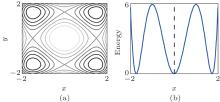
We first illustrate the RED in two simple toy models. The first one is a two-dimension (2D) system with four identical potential wells, denoted as Two-Dimension-Quad-Well (TDQW), see Fig. 1(a). The second model is a 2D system with a Mexican– Hat potential (MHAT) which has two states, see Fig. 1(b). The outer state is wide (larger entropy) and the relaxation time inside the state is comparable to the transition time between the state and the inner state. Simulation details and the applied basis functions are shown in Appendix A.
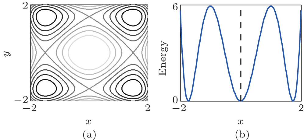 | Fig. 1. The 2D potentials. (a) The TDQW potential shown as contour map. The darker regions correspond to potential wells, and the lighter regions correspond to potential barriers. (b) The MHAT potential projected along one dimension. Rotating around the dashed line reproduces the 2D potential. |
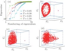
In TDQW system, the eigenvalues of the matrix H in Eq. (6) are plotted in Fig. 2(a). As expected, there are four zero eigenvalues at temperature 0.3, implying the four disconnected states. At higher temperatures, the second to fourth eigenvalues deviate from zero to larger values due to the increasing fraction of the interstate transition trajectories. More illustrative perspective can be obtained from Figs. 2(b), 2(c), and 2(d), where the trajectories are mapped into the three-dimensional space by projecting the trajectory-mapped vectors, {Gi} defined in Eq. (7), to the second, third, and fourth eigenvectors of H, denoted as
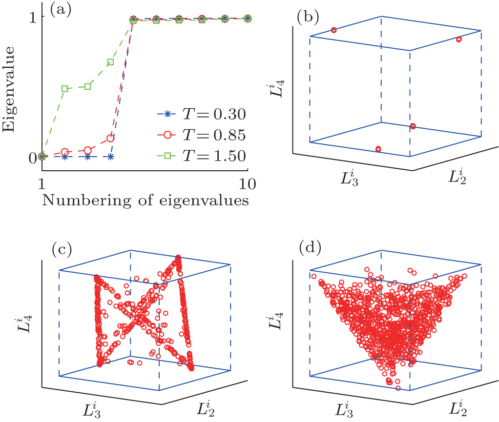 | Fig. 2. The eigenvalues and projection maps for TDQW potential under different temperatures. (a) The first ten eigenvalues of H matrix calculated at different temperatures. For the three temperatures of 0.3 (b), 0.85 (c), and 1.50 (d), the projection of {Gi} to the second, third, and fourth eigenvectors of H are also plotted. |
In MHAT system, the 70 smallest eigenvalues of H are shown in Fig. 3(a). Different from TDQW, the eigenvalues of H gradually increase from zero at the low temperature T = 0.05, and lots of small eigenvalues exist. The number of the eigenvalues that obviously deviate from 1.0 is always more than the number of physical states in MHAT system, till the temperature is high enough that there is only one zero-eigenvalue apparently different from 1.0. This behavior simply reflects the entropic nature of the outer potential well. At low temperature, a single trajectory cannot reach local equilibrium in the state, consequently a few small eigenvalues exist, as there are many sub-states in the well. At higher temperatures, the trajectories that start from the outer potential well usually climb over the potential barrier before reaching local equilibrium within the state, thus the inter-trajectory difference will not be extinguished, until the two states in MHAT kinetically become one state at high enough temperature. The projections of {Gi} onto the eigenvectors of H are shown in Figs. 3(b), (3c), and 3(d). At both temperatures 0.05 and 0.30, the trajectories are divided into two groups. In one group, the trajectories dispersively locate on the same plane which is perpendicular to the 
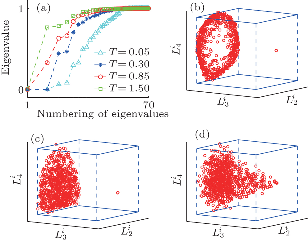 | Fig. 3. The eigenvalues and projection maps for MHAT potential under different temperatures. (a) The first seventy eigenvalues of H matrix calculated at different temperatures. For the three temperatures of 0.05 (b), 0.30 (c), and 0.85 (d), the projection of {Gi} to the second, third, and fourth eigenvectors of H are also plotted. |
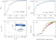
In the two 2D models, triangle functions in the 2D space are applied as basis functions, and the details are presented in Appendix A. We did the S2 analysis mentioned in Subsection 2.2 at T = 0.85. For both systems, S2 initially grows fast with increasing number of basis functions, then the growth slows down and shows a saturation behavior of S2 as expected [see Figs. 4(a) and 4(b)]. Once S2 has approximately reached the platform region, more basis functions will not change the calculation results anymore (data not shown). Thus, for TDQW and MHAT systems, about 24 basis functions are sufficient.
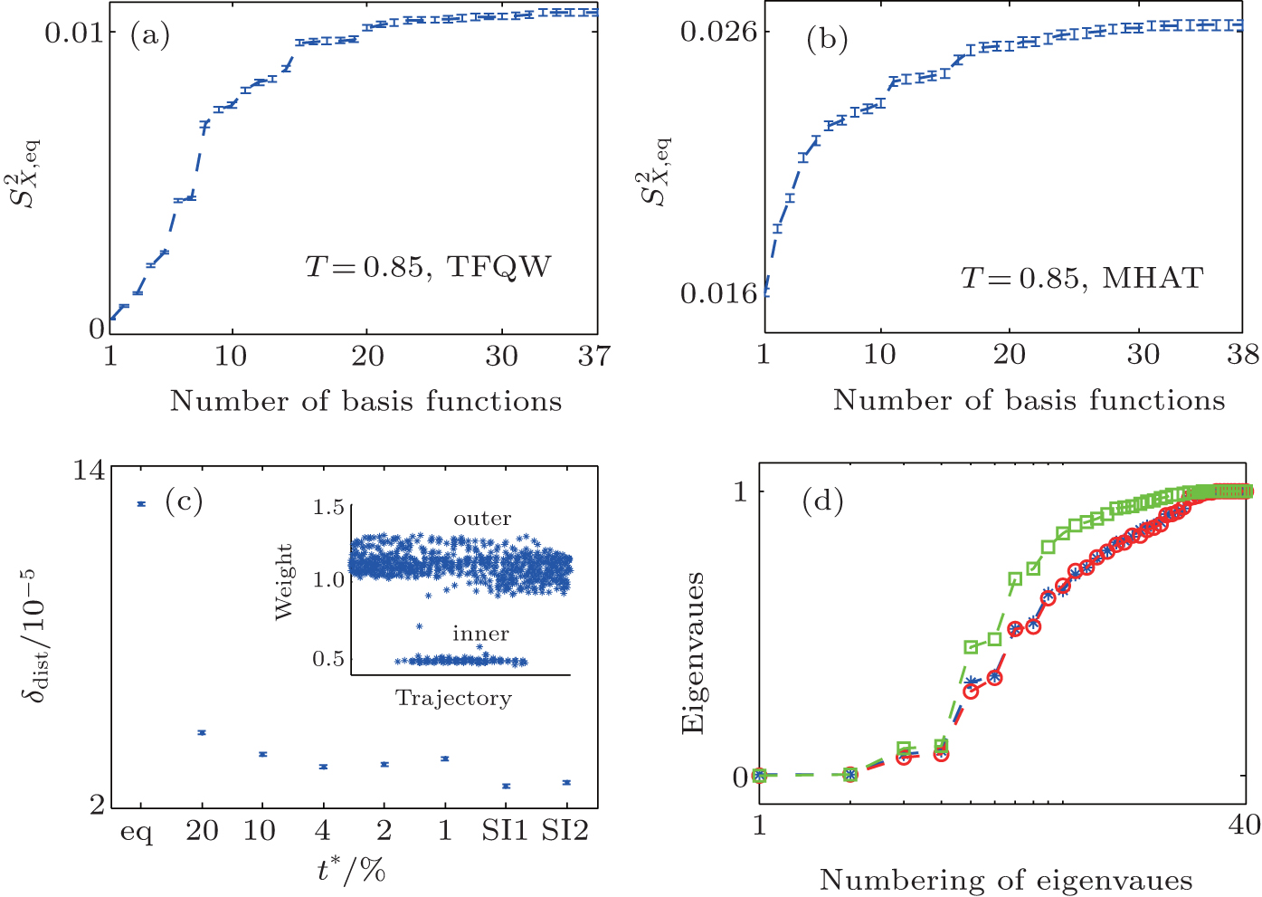 | Fig. 4. The S2 curve, effect of t̃ , and illustration of statistics improvement. The behavior of S2 with increasing number of basis functions are shown in panel (a) (TDQW) and panel (b) (MHAT). (c) The difference between the reconstructed equilibrium distribution and the theoretical distribution are shown for MHAT potential at T = 0.85. The horizontal axis denotes the method for reproducing the equilibrium distribution. ‘ eq’ means the results without reweighting (i.e., wi = 1), numbers mean the selected   |
We also study the effect of free parameter t̃ in the RED with the simulation data of MHAT at T = 0.85. In this case, since there is only one zero eigenvalue of H, the whole free energy surface can be reconstructed. We uniformly divide the whole conformational space into small cells, k = 1, … , Np (Np is selected as 1600 here, i.e., 40 bins along each dimension), and the distribution probability in each cell is reconstructed with different 


to measure the difference between the reconstructed distribution and the theoretical distribution. Here 


We test the statistics improvement methods, SI1 and SI2. In here and below, we always randomly select one-fifth of the initial configurations, then five trajectories are spawned from each configuration to test the improvement. At T = 0.85, we apply both SI1 and SI2 to reconstruct the energy surface of MHAT. From Fig. 4(c), it can be seen that both methods correctly reproduce the energy surface with even smaller deviation from the theoretical one, as compared to the standard RED. At T = 0.05, the eigenvalues of the H matrix are calculated with SI2 method. As shown in Fig. 4(d), no matter whether one trajectory or multiple trajectories are generated from one initial configuration, the eigenvalues calculated by the standard RED are almost the same. However, analyzing by the SI2 method significantly alters the structure of eigenvalues. By generating more trajectories from single initial configuration, and combining these trajectories together in analysis, the statistics of the single trajectory are prominently improved, and the difference between trajectories within the outer state are reduced to a large extent. As a result, some of the eigenvalues increase, in particular for the ones deviating but close to 1.0. In other words, the SI2 method has depressed the statistical noise in the spectral analysis of H, leaving the physically relevant states recognized.
The simulated system together with the initial configurations of simulation are shown in Fig. 5, where various notations of the atoms, dihedral angles, and free energy wells of this molecule are introduced. More details of simulations are presented in Appendix B.We use two different classes of basis functions to focus on the effects of different physical variables on the observed metastable states.
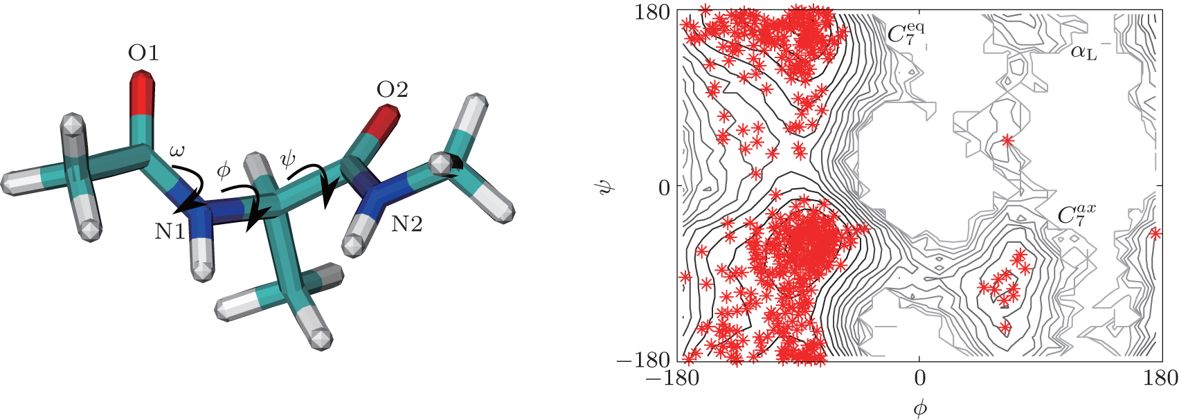 | Fig. 5. Illustration of the alanine dipeptide molecule and the initial conformations of the RED simulation. The alanine dipeptide is shown in the left panel, with some dihedral angles and atoms labeled. The initial conformations projected to the ϕ – ψ plane are shown in the right panel. The background is the free energy surface at T = 600 K, with the free energy wells labeled. |
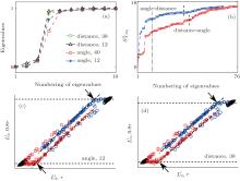
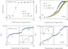
With thorough investigation, the two dihedral angles ϕ and ψ are the major coordinates to characterize the conformational motion of the alanine dipeptide molecule. As in the previous study, [35] we adopted the first-to-fourth order twodimensional trigonometrical functions of ϕ and ψ as the basis functions. The 10 smallest eigenvalues of H are shown in Fig. 6(a). The smallest zero eigenvalue is intrinsic due to the construction of H. The second eigenvalue corresponds to the kinetic separation between the region with ϕ > 0 (containing 


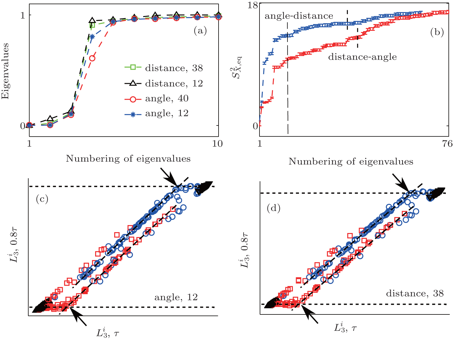 | Fig. 6. RED analysis with the basis functions of dihedral angles and inter-atomic distances. Shown are the results for solvated alanine dipeptide, which is simulated at T = 300 K with the modified force field. (a) The eigenvalues of H matrix calculated with different sets of basis functions, including the full set of inter-atomic distances (squares), 12 inter-atomic distances (upward triangles), first-to-fourth order trigonometrical functions of ϕ and ψ (circles), and first-to-second order trigonometrical functions of ϕ and ψ (stars). (b) The behavior of S2 is shown either with the inter-atomic distances (distance-angle) at first, or with the trigonometrical functions of ϕ and ψ at first (angle-distance). The  |
We also test the effects of distances between atoms in the backbone of dipeptide by using them as basis functions. We compare two aspects, i.e., the eigenvalues of H and the manipulations on 


| Table 1. Basis function list. |
We also apply the RED to study the low-temperature (T = 150 K) properties of the dipeptide. We note that, at this temperature, the physical phenomena are quite complicated; the force field and the simulation procedure that we adopt may not reflect the physical reality. Here, we are only meant to illustrate the application of the RED in the extreme condition, instead of providing physical insight into the system.
The eigenvalues of the H matrix are calculated with the 91 basis functions listed in Table 1, and are plotted in Fig. 7(b). The solvent-related quantities do affect the eigenvalues of H now, leading to even more small eigenvalues. Correspondingly, the S2, as shown in Fig. 7(d), almost always increases with the number of basis functions. At such a low temperature, the free energy surface becomes quite rough, and the diffusive dynamics[39] in the conformational space slows down seriously. As a result, the simulation trajectories may only explore a small region in the conformational space. Some degrees of freedom, like the solvent motion around the solute molecule and the conformational motion perpendicular to the ϕ – ψ plane, are no longer equilibrated in a single trajectory. Thus, the inter-trajectory difference becomes larger, more states are detected automatically, and more basis functions are required to expand the rugged distribution of the samples, leading to the abnormal behavior of the eigenvalues of H and S2.
Manipulating the eigenvectors of H can provide further information of the simulation data. The projections of {Gi} to the second and the third eigenvectors of H pick out two completely separated states, 


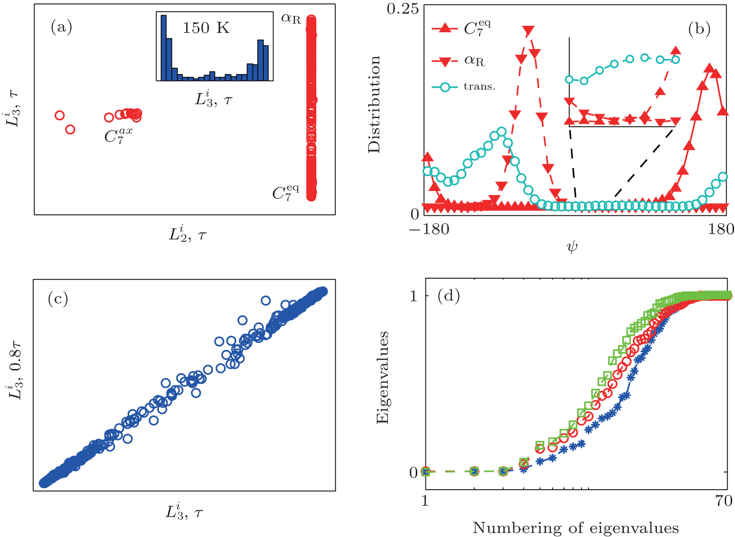 | Fig. 8. Results for the low-temperature simulation of alanine dipeptide. (a) The projection of trajectories into the space of     |
Due to the numerous local minimums at the low temperature, the α R and 
As a summary, in the dipeptide system at T = 300 K with modified potential, we find the redundant basis functions (including functions of both the dihedral angles and the inter-atomic distances) are consistently treated in the RED, and the inclusion of the solvent-related basis functions gives out the expected results. At pretty low temperature of 150 K, the roughness of the free energy surface is reflected in the results of RED. The conformational space can still be roughly divided into parts, however, the kinetics becomes too complicated to be unambiguously characterized.
As a systematic method for exploring the conformational space, the RED does not require much a priori knowledge and approximation, thus its results can honestly reflect the thermodynamic and kinetic information of the system. For biological macromolecules, the usually expected hierarchical structure can be extracted out step-by-step. For these complex systems, the structure of the conformational space may be much more complicated, these examples studied here become quite relevant for physically interpreting the results. Along with the applications, we design the S2 quantity for checking the completeness of the selected basis functions, and the schemes for statistics improvement. These tactics are also proved to be helpful for portraying the conformational space.
Zhou Xin is grateful for the financial support of the Hundred of Talents Program in the Chinese Academy of Sciences. Gong Lin-Chen and Zhou Xin are also grateful for the support of the Max Planck Society and the Korea Ministry of Education, Science and Technology; part of the work was done while they worked at the Asia Pacific Center for Theoretical Physics, Korea under this support.
| 1 |
|
| 2 |
|
| 3 |
|
| 4 |
|
| 5 |
|
| 6 |
|
| 7 |
|
| 8 |
|
| 9 |
|
| 10 |
|
| 11 |
|
| 12 |
|
| 13 |
|
| 14 |
|
| 15 |
|
| 16 |
|
| 17 |
|
| 18 |
|
| 19 |
|
| 20 |
|
| 21 |
|
| 22 |
|
| 23 |
|
| 24 |
|
| 25 |
|
| 26 |
|
| 27 |
|
| 28 |
|
| 29 |
|
| 30 |
|
| 31 |
|
| 32 |
|
| 33 |
|
| 34 |
|
| 35 |
|
| 36 |
|
| 37 |
|
| 38 |
|
| 39 |
|
| 40 |
|