


Neural adaptive chaotic control with constrained input using state and output feedback*
Cite this Article
Gao Shi-Gen, Dong Hai-Rong, Sun Xu-Bin, Ning Bin. Neural adaptive chaotic control with constrained input using state and output feedback* . Chinese Physics B, 2015, 24(1): 010501 
Permissions
Neural adaptive chaotic control with constrained input using state and output feedback*
Corresponding author. E-mail: hrdong@bjtu.edu.cn
Project supported by the National High Technology Research and Development Program of China (Grant No. 2012AA041701), the Fundamental Research Funds for Central Universities of China (Grant No. 2013JBZ007), the National Natural Science Foundation of China (Grant Nos. 61233001, 61322307, 61304196, and 61304157), and the Research Program of Beijing Jiaotong University, China (Grant No. RCS2012ZZ003).
Abstract
This paper presents neural adaptive control methods for a class of chaotic nonlinear systems in the presence of constrained input and unknown dynamics. To attenuate the influence of constrained input caused by actuator saturation, an effective auxiliary system is constructed to prevent the stability of closed loop system from being destroyed. Radial basis function neural networks (RBF-NNs) are used in the online learning of the unknown dynamics, which do not require an off-line training phase. Both state and output feedback control laws are developed. In the output feedback case, high-order sliding mode (HOSM) observer is utilized to estimate the unmeasurable system states. Simulation results are presented to verify the effectiveness of proposed schemes.
Keyword:
05.45.Gg; chaotic control; neural adaptive control; constrained input
1. Introduction
In recent years, chaotic control has aroused considerable concern after the findings of Lorenz system, [1]
In Ref. [20], a feedback linearization control is applied to control a chaotic pendulum system considering the presence of saturation in control signals, the stability of the controller is investigated in the presence of saturation, and corresponding sufficient stability conditions are obtained. In Ref. [21], an adaptive sliding mode control scheme for Lorenz chaos subject to saturating input is presented. In Ref. [22], backstepping-based adaptive fuzzy neural controller control of unknown chaotic systems with input saturation is given, the auxiliary system with the same order as that of the plant[23] is used to deal with saturation. It is noticeable that the methods in these works are developed using available system states, which may restrict the real applications in practical engineering in which sometimes only system output information is available for control design. Furthermore, the method in Ref. [23] suffers from the problem of “ explosion of complexity” , which is caused by the repeated differentiations of the so-called “ virtual” controls. Although dynamic surface control technique[24] can be used to solve this difficult point, the backstepping design requires tedious and complex analysis.[25] As reported in Ref. [26], direct current motor control is a relatively simple application, but the regression matrix in the adaptive backstepping control almost covers an entire page in Ref. [27].
In this paper, neural adaptive control is developed for a class of chaotic nonlinear systems subject to unknown dynamics and constrained input. Radial basis function neural networks (RBF-NNs) are used to online approximate unknown nonlinear dynamics, the auxiliary system similar to Refs. [22] and [23] is used to generate signals which attenuate the effect of input saturation. The new features of the developed methods compared to Refs. [22] and [23] contain two aspects: (i) by virtue of properly selected state vector and constructed auxiliary system, backstepping used in Ref. [22]) is not used in this paper; (ii) both state and output feedback cases are considered in this paper. In the output feedback case, HOSM observer[31] is utilized to estimate the unmeasurable system states. The prominent feature of the HOSM observer lies in that it guarantees finite-time observer error convergence and therefore is an admirable tool for feedback control design with separation principle trivially satisfied.
2. Problem formulation and preliminaries
Consider a class of uncertain chaotic systems in the following form:
 |
where 
 |
where u+ denotes the bound of the serving actuator.
The objective is to design a proper control u such that: (i) the closed-loop system is semi-globally stable in the sense that all the signals are ultimately uniformly bounded; (ii) the output of chaotic system y = x1 tracks the desired signal yr with adjustable tracking error.
To this end, the following lemma and assumptions are used to design a feasible control law.
Lemma 1[33] An unknown smooth function F(Z) can be approximated by RBF NNs as F(Z) = WTS(Z), where Z ∈ Ω Z ⊂ Rq is the input to the neural network, with q being the NN input dimension, W = [w1, w2, … , wl]T is the adjustable parameters vector, l is the number of neurons, S(Z) = [s1(Z), s2(Z), … , sl(Z)]T, with si(Z) being Gaussian functions, i.e., si(Z) = exp(− (Z – μ i)T(Z – μ i)/η i2), i = 1, 2, … , l, where μ i and η i denote the centers and widths of the Gaussian functions, respectively. As indicated in Ref. [34], by setting a large enough number of hidden neurons, the RBF NNs are capable of approximating F(Z) to arbitrary accuracy over a compact set Ω Z ⊂ Rq

where W* is the so-called “ optimal” bounded weight vector which minimizes ε (Z)

with ε (Z) being the bounded approximation error, and | ε (Z)| ≤ ε *.
Assumption 1 The optimal neural weight vector W* is bounded by unknown constant ‖ W*‖ ≤ W+ , and W+ > 0 is an unknown constant. The Gaussian basis function vector S(Z) is also bounded, i.e., ‖ S(Z)‖ ≤ S* with S* > 0 being an unknown constant.
Assumption 2 The desired signal yr and its derivatives up to the n-th order are known and bounded.
Assumption 3[36] The system (1) is input-to-state stable.
Remark 1 As indicated in Ref. [35], it is extremely hard to obtain general stability conditions for general unstable systems with input saturation. Therefore, Assumption 3 is used in Ref. [36] to develop feasible control law. In this paper, Assumption 3 implies that the chaotic systems considered are stable, since the actual input to the system is always bounded by saturation, the boundedness of states are guaranteed, which will facilitate the stability analysis in the following analysis.
3. Control design
3.1. Neural adaptive control using state feedback
Define the following vectors:

where ζ ∈ Rn is an auxiliary signal vector generated by the following constructed system:
 |
where κ 1, κ 2, … , κ n are design parameters, and Δ u: = v– u.
Remark 2 By setting the initial value of ζ as 0, the auxiliary system given in Eq. (3) has no response without input saturation, i.e., Δ u = 0. When saturation happens, a sudden rise will appear in 
Introduce a filtered tracking error as follows:
 |
where Λ = [λ 1, λ 2, … , λ n– 1]T, λ i (i = 1, 2, … , n– 1) are chosen such that the polynomial sn– 1 + λ n– 1sn– 2 + … + λ 1 is Hurwitz. In this sense, one can guarantee boundedness of 𝑒 with bounded 𝒮 .
The designed neural adaptive control for chaotic system described by Eq. (1) is given in the following theorem.
Theorem 1 Consider the chaotic system described by Eq. (1). If a neural adaptive control with weight adaptation laws are designed as follows:

 |
where k1 > 0 is a design parameter, K = diag{κ 1, κ 2, … , κ n} is a diagonal matrix, where κ 1, κ 2, … , κ n are design parameters defined in Eq. (3). Γ 1 = Γ 1T > 0 is adaptive gain matrix, Ŵ 1 is the estimated value of (i) All the signals in the closed-loop system are uniformly ultimately bounded. (ii) The transient performance of tracking error between system output y and reference signal yr with input saturation in effect satisfies the following inequalities:

where

and

and V1(0) is the initial value of V1(t)| t = 0.
Proof Considering the open-loop dynamics (4) and control laws (5), the closed-loop dynamics is obtained as
 |
where 

Consider the following Lyapunov candidate:
 |
its derivative along the adaptation laws can be calculated by
 |
Define τ 1 = min{k1, σ 1/2}/ max{1/2, ‖ Γ 1− 1‖ /2} and 


implying that there exists a moment T such that for any t > T, one has


When the input saturation is in effect, the solution of Eq. (3) can be obtained as 

3.2. Neural adaptive control using output feedback
In this section, neural adaptive control is designed using output feedback, i.e., only y can be used in the control design. To this end, a high-order sliding mode observer named Levant's differentiator is utilized, as described in the following lemma.
Lemma 2[31]Levant's differentiator Consider a signal ℒ (t) defined in the range of [0, ∞ ], which is composed of a bounded noise and an unknown base signal ℒ 0(t), with the noise being Legesgue measurable and the n-th derivative of base signal ℒ 0(t) having a known Lipschitz constant L > 0. The following constructed high-order sliding mode observer, with β i (i = 1, 2, … , n) being positive constants selected by the designers:
 |
guarantees that (i) there exists a time moment T, such that for any t> T, one obtains 


Remark 3 Lemma 2 means that equation (9) is kept in two-sliding mode, i.e., 

By virtue of the property of the above-mentioned observers,


therefore, 

The designed output feedback neural adaptive control using sliding-mode observer is given in the following theorem.
Theorem 2 Consider the chaotic system described by Eq. (1). If a neural adaptive control with weight adaptation laws are designed as follows:
 |
where k2 > 0 is a design parameter, (i) All the signals in the closed-loop system are uniformly ultimately bounded. (ii) The transient performance of tracking error between system output y and reference signal yr with input saturation in effect satisfies the following inequalities:


where 

Proof Consider a Lyapunov function 
 |
It is clear that 


The closed-loop system is governed by
 |
where 

Consider a Lyapunov function 
where 

Remark 4 Since the approximation property of RBF NNs in Lemma 1 is only guaranteed in the compact set specified by Ω Z, the stability results in this work, therefore, are semi-global. In this sense, a reasonable suggestion, i.e., small sets of initial values of NN weights and tracking error, is made to the ones who want to put the main results of this work into practice.
4. Simulation results
To evaluate the developed algorithms for controlling chaotic systems, we consider two nonlinear chaotic systems, i.e., Duffing system and Arneodo system. To simulate the measurement noise when applying Theorem 2, a random number with proper amplitude is added to the observer input signal in each discrete time computation, which is rough enough to mimic measurement noise. The sample time used in the simulation is Δ T = 10− 4, without proper designed control scheme, the amplitude of noise is potentially amplified by 104 and 108 times for two- and three-order systems in discrete time calculation.
4.1. Duffing system
Consider the following Duffing system, [29] whose chaotic behavior is shown in Fig. 1.
 |
Theorem 1 and Theorem 2 are applied to the Duffing system to control the output to track the reference signal yr = sin(t) with constrained input specified by u+ = 12. The design parameters are set as follows: k1 = k2 = 15, κ 1 = 6, κ 2 = 8, Λ = 5, Γ 1 = Γ 2 = I, and σ 1 = σ 2= 0.001. The neural networks contain 41 nodes with centers evenly spaced on [− 2, 2] and widths are all 1. Initial values of x1, x2, ζ 1, and ζ 2 are 0.6, 0.15, 0, and 0, respectively. Initial values of neural network weights are all 0. The parameters of the HOSM observer are β 1 = 12, β 2 = 15, and β 3 = 20. The noise is added to the observer in the form of ω = α · rand [− 0.5, 0.5], with α = 0.01 in this case.
Simulation results of controlling Duffing system are presented by Figs. 2– 6. Figure 2 presents the tracking performance and tracking errors in controlling Duffing system, and the state x2 of the controlled Duffing system is shown in Fig. 3. Signals generated by constructed auxiliary system are shown in Fig. 4, while figure 5 presents the observer errors using Theorem 2. The boundedness of control inputs are shown in Fig. 6. It is observed that all the closed-loop signals are bounded and the performance is satisfactory.
 | Fig. 1. Chaotic behavior of Duffing system. |
 | Fig. 2. (a) Tracking performance of Duffing system (dashed line: output using Theorem 1, solid line: reference signal, dot-dashed line: output using Theorem 2). (b) Tracking errors (dashed line: error using Theorem 1, dot-dashed line: error using Theorem 2). |
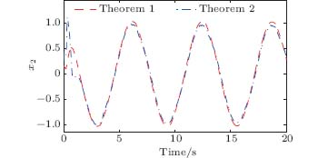 | Fig. 3. State x2 of controlled Duffing system. |
 | Fig. 4. Trajectories of (a) ζ 1 and (b) ζ 2. |
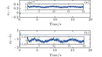 | Fig. 5. Observer errors (a)   |
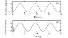
 | Fig. 6. Control inputs in controlling Duffing system. (a) Theorem 1; (b) Theorem 2. |
4.2. Arneodo system
Consider the following Arneodo system, [30] whose chaotic behavior is shown in Fig. 7.
 |
The reference signal is also yr = sin(t) with u+ = 12. The design parameters here are as follows: k1= k2= 5, κ 1 = 9, κ 2 = 8, κ 3 = 7, Λ = [35 12]T, Γ 1= Γ 2= I, and σ 1= σ 2= 0.001. Other settings are the same as the above subsection. The parameters of the HOSM observer are β 1 = 10, β 2 = 15, β 3 = 18, β 4 = 5, and α = 0.001.
 | Fig. 7. Chaotic behavior of Arneodo system. |
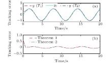
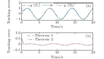 | Fig. 8. (a) Tracking performance of Arneodo system (dashed line: output using Theorem 1, solid line: reference signal, dot-dashed line: output using Theorem 2). (b) Tracking errors (dashed line: error using Theorem 1, dot-dashed line: error using Theorem 2). |
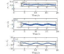
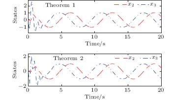 | Fig. 9. States x2 and x3 of controlled Arneodo system. |
Simulation results of the controlling Arneodo system are presented by Figs. 8– 12. Figure 8 presents the tracking performance and tracking errors in controlling Arneodo system, and the states x2 and x3 of controlled Arneodo system are shown in Fig. 9. Signals generated by constructed auxiliary system are shown in Fig. 10, while figure 11 presents the observer errors using Theorem 2. The boundedness of control inputs are shown in Fig. 12. Clearly, the tracking performance is satisfactory in controlling Arneodo system as well.
From the aforementioned theoretical analysis and simulation results of both cases, we can conclude that the developed control schemes are valid for a class of uncertain chaotic nonlinear systems with constrained input.
 | Fig. 10. Trajectories of (a) ζ 1, (b) ζ 2, and (c) ζ 3. |
 | Fig. 11. Observer errors (a)  |
 | Fig. 12. Control inputs in controlling Arneodo system. (a) Theorem 1; (b) Theorem 2. |
5. Conclusions
This paper has developed neural adaptive control schemes for a class of chaotic nonlinear systems in the presence of constrained input and uncertain dynamics. RBF NNs are used in the online learning of uncertain dynamics. To attenuate the effect caused by constrained input, an auxiliary system with the same order as that of the plant is constructed to generate signals to compensate the effect of input saturation. Except showing the stability of closed-loop system, transient performance with input saturation in effect is obtained rigorously in terms of design parameters. Applications of the developed methods to Duffing system and Arneodo system to track a reference trajectory. Simulation results show that the methods developed perform successful control and achieve desired performance.
Reference
| 1 |
|
| 2 |
|
| 3 |
|
| 4 |
|
| 5 |
|
| 6 |
|
| 7 |
|
| 8 |
|
| 9 |
|
| 10 |
|
| 11 |
|
| 12 |
|
| 13 |
|
| 14 |
|
| 15 |
|
| 16 |
|
| 17 |
|
| 18 |
|
| 19 |
|
| 20 |
|
| 21 |
|
| 22 |
|
| 23 |
|
| 24 |
|
| 25 |
|
| 26 |
|
| 27 |
|
| 28 |
|
| 29 |
|
| 30 |
|
| 31 |
|
| 32 |
|
| 33 |
|
| 34 |
|
| 35 |
|
| 36 |
|