Two-dimensional (2D) materials of honey-lattice structure are expected to exhibit new quantum states, including new spin-valley structures and characteristic edge states, when some of the symmetries of the system are broken. Graphene has two degenerate and inequivalent valleys at opposite corners of the Brillouin zone and the valley degree of freedom is assumed to be a carrier of information.^{[1, 2]} When graphene is subjected to a strong magnetic field, it exhibits a sequence of integer quantum-Hall platforms at filling factors ν = ± g(n + 1/2), where g = 4 results from the spin and valley degeneracy.^{[3, 4]} The n = 0 Landau level (LL) is of particularly interest, since it has only one electron-like and holelike dispersive edge state for a given spin and edge. In an extremely high magnetic field, the insulating state ν = 0 is observed at the Dirac point, ^{[5– 7]} which indicates that the n = 0 LL should split into several sublevels due to the broking of the sublattice and spin degeneracies by the staggered potential and Zeeman energy. Several scenarios have been put forward to explain the ν = 0 insulating state, including the charge density wave, ^{[8– 10]} the Kekule distortion, ^{[11, 12]} the ferromagnetic (FM), ^{[13, 14]} the antiferromagnetic (AF), ^{[10, 15]} and the canted antiferromagnetic (CAF) states.^{[16– 19]}

A recent experimental breakthrough by Young et al.^[20] has shown that the ν = 0 state would turn into a metallic phase at strong magnetic field. At a weak magnetic field B, the ν = 0 state is insulating with the system’ s conductance G = 0. As the magnetic field B increases, the ν = 0 state changes from the insulator phase to a phase with thermally activated edge transport and the conductance is G ≈ e²/h. At a higher B, the system is evolved into a phase with G slightly below 2e²/h. Moreover, the new quantum states with half-integer conductances (1/2e²/h, 3e²/2h) were also observed by varying a gate voltage. These findings showed that the Zeeman energy (M = gμ _BB) may play a significant role in the formation of new quantum states. The quantum phase transition of the ν = 0 state has been investigated by many authors from several different aspects, ^{[21– 23]} such as the competition between the magnetic field-driven Peierls-type lattice distortion and random bond fluctuations; ^[23] however, the properties of the halfinteger metal states including the charge-spin-valley structure and the edge-state characters discerned in silicene^{[24– 27]} are untouched in graphene.

In this work, we will study possible quantum Hall states of graphene in a magnetic field by considering the Zeeman splitting M and the lattice staggered potential Δ and interpret the experimental observations.^[20] The lattice staggered potential results from a graphene– substrate interaction, ^{[5– 7, 20]} such as when graphene is grown on the h-BN substrate it will produce such interaction, so the inversion symmetry of graphene is broken and the valley degeneracy of graphene^{[28, 29]} is lifted. Moreover, in a strong magnetic field case, the Zeeman splitting cannot be neglected and it has already been demonstrated in the quantum capacitance measurements.^{[30, 31]} By taking these two factors into account, we have shown that there are abundant quantum Hall phases emerging in the system, depending on the system parameters. When M < Δ , the quantum valley Hall (QVH) phase appears, with the edge states from opposite valleys propagating in opposite transverse edges. Although the conductance G = 0, it is really different from a band insulator phase because it has a QVH conductance, which may be detected in experiments.^{[32, 33]} As M > Δ the quantum spin Hall (QSH) phase emerges with the two spin species propagating along the edges in opposite directions, leading to a G = 2e²/h conductance. This QSH state resulting from spin polarization has fundamental difference with the QSH state originating from the spin– orbit coupling (SOC) although they have the same features, because it consists of electron- and hole-like copies of the quantum Hall effect, which has opposite spin polarizations and is protected by the spin conservation rather than the time-reversal symmetry as in the systems with strong SOC.^[20] When the Fermi energy deviates from the Dirac point, there is a quantum charge-spin-valley Hall (QSVH) phase with a unity conductance. The boundary state connecting two neighboring quantum Hall phases was shown to be metallic with a half-integer conductance.

We first consider a continuum model describing lowenergy Dirac electrons in graphene. In a perpendicular magnetic field B, the effective Hamiltonian with a Zeeman field strength M and lattice potential Δ is given by:^{[33, 34]}

Here τ _z = ± 1 for the K and K′ valleys, (A_x, A_y) are the components of the magnetic vector potential, υ _F characterizes the Fermi velocity of Dirac fermions and was set ħ υ _F = 1 in the following calculations. σ = (σ _x, σ _y, σ _z) are the Pauli matrices representing the lattice pseudospin, s_z is a real spin index. Using the Landau gauge field A = (0, Bx, 0), the Landau levels of Dirac electrons in graphene are given by for n ≠ 0 and for n = 0, where is the cyclotron frequency, s = + /− denotes electrons/holes, and n is an integer.

In Ref. [24], the Chern and spin-Chern numbers were adopted to depict the quantum phases in the silicene system while they are ill-defined in the valley-polarized metal state since the Fermi energy locates in the bulk. In our model, we will not calculate the flavor Chern number characterizing each phase and, instead, we will use the Hall conductivity to describe possible topological phases in graphene. Certainly, these two cases are equivalent in labeling a quantum state and, moreover, one can even use the Hall conductivity to define a metallic state.

Taking the same procedure as Refs.  [34]– [36], we can use the standard Kubo formula to calculate the Hall conductivity . Near the Dirac point, the spin s_z and valleys τ _z Hall conductivity is given by

Here represents the Fermi– Dirac distribution function of the n-th LL with spin s_z from K (K′ ) valley for electron-like particles (s = + ) or hole-like particles (s = − ). The total Hall conductivity is the sum of Hall conductivity from the two valleys . Also, the spin and valley Hall conductivities can be written as and . The Hall conductivities near the Dirac point rely on which Landau level is occupied. For instance, as Δ = 0 and a finite Zeeman energy M, the n = 0 LL is spin-splitting and the two n = 0 spin LLs move up and down oppositely. In the energy interval between the two LLs, because only is occupied while because only is empty. Subsequently, a set of quantum number is obtained (we set e²/h = 1 for simplicity) which represents the QSH phase.

In order to describe different quantum Hall states, we will calculate the spatial distribution of the edge state characterizing each quantum Hall phase. In the tight-binding representation, the Hamiltonian for graphene in the presence of magnetic field and staggered potential is given by

where and a_iα are the creation and annihilation operators at the discrete site i with spin polarization α , and 〈 i, j〉 runs over all the nearest neighbor hopping sites. The first term represents the on-site energy, the second term represents the nearest neighbor coupling, and the last two terms stand for the lattice potential and the Zeeman energy, respectively. In the presence of magnetic field B, a Peierls phase factor ϕ _ij is added in the hopping interactions, and with the vector potential A = (0, Bx, 0) and ϕ ₀ = ħ /e.

In the following section, we will discuss possible quantum Hall phases characterized by the quantum number according to Eq.  (2) and the properties of the edge states. In the numerical calculations, we consider a zigzag edge graphene nanoribbon with 96 atoms in a unit cell. Under a perpendicular magnetic field B, the magnetic flux through a honeycomb lattice is and we set the corresponding Peierl’ s phase to .

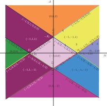
We first consider the Fermi energy located at the Dirac point and calculate all possible quantum phases in the M– Δ parameter space. The phase diagram is shown in Fig.  1 and in this case the quantum phases are well known: there are QSH phases with (0, ± 2, 0) for | M| > | Δ | , QVH phases with (0, 0, ± 2) for | M| < | Δ | , and QSVH phases with (0, ± 1, ± 1) at the phase boundaries. Actually, the QSVH phase here is strictly not a quantum Hall state and, instead, it is a metallic state since it is the boundary state connecting the neighboring QSH and QVH phases. The QSH state is not due to the spin– orbit interaction but is due to the Zeeman splitting. Since the electron-like and hole-like particles have opposite Hall coefficients, a nonzero quantum spin Hall current can flow in the graphene due to the Zeeman splitting.

Fig.  1.

	Figure Option ViewDownloadNew Window
	Fig.  1. Phase diagram in the M– Δ panel with Fermi energy at the Dirac point. Heavy lines represent phase boundaries, which represents the points where the Fermi energy Ef crosses the flat part of the energy band. A number shows a point where the energy spectrum is calculated and shown in Fig.  2.

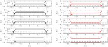
In order to distinguish each quantum phase we will study the electronic band structures and edge-state properties based on a finite single-layer graphene model with zigzag edges. Figure  2 shows the spin-dependent band structure in the low energy region, which corresponds to numerals 2 and 3 in Fig.  1. When M > Δ (the phase 3), the spin-up hole edge states and spin-down electron edge states cross the Fermi energy E_f. From

one can find that states A  (B) and D  (C) propagate along the same + x  (− x) direction.^[37] When M = Δ (2 point in Fig.  1), the Fermi energy exactly crosses the flat part of the spin-up hole band and spin-down electron band, and the two states from E and F propagate along the + x direction.

Fig.  2.

	Figure Option ViewDownloadNew Window
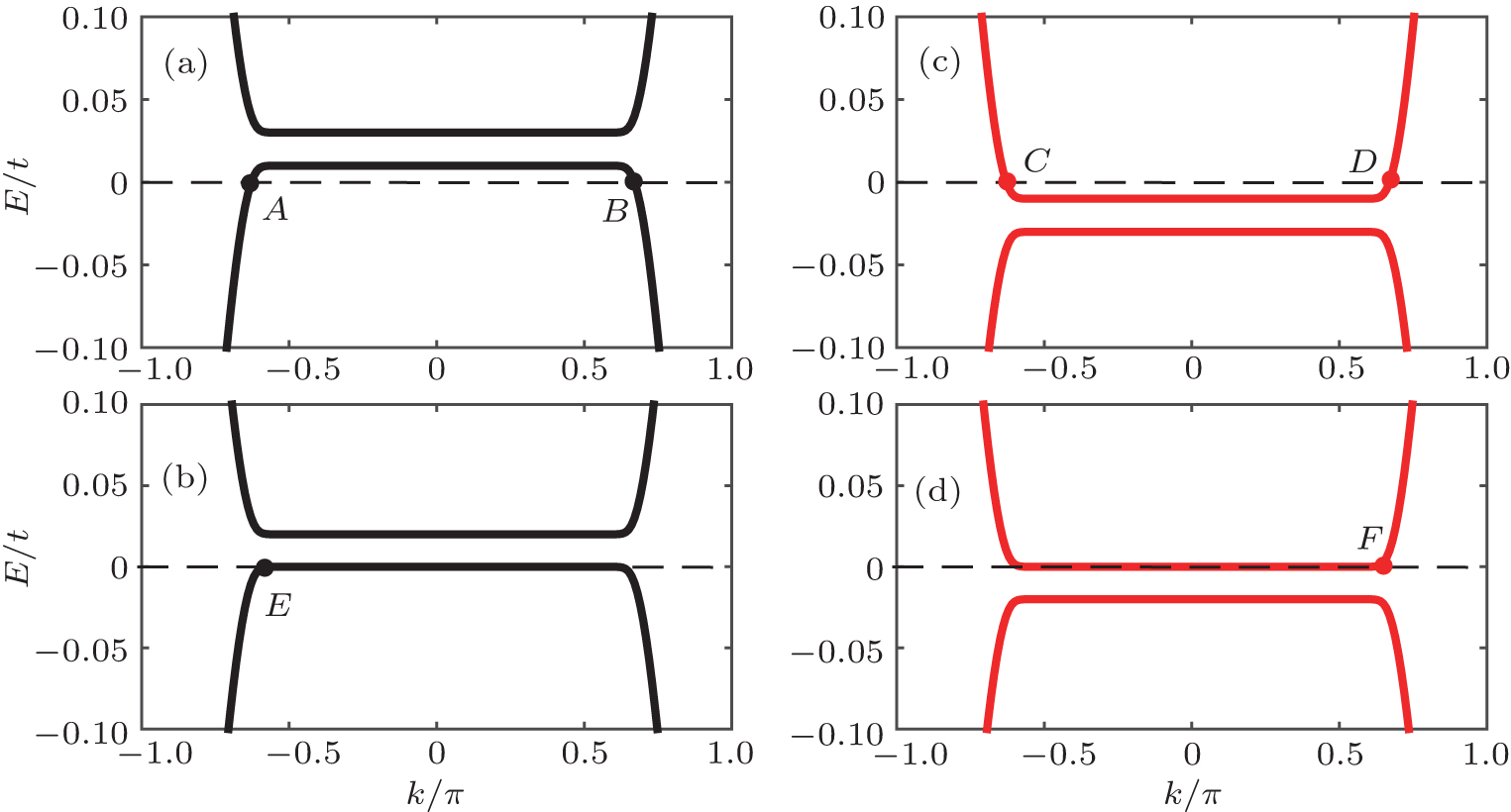	Fig.  2. Edge-state band structure of the spin-up (black lines) and spin-down (red lines) electron of a zigzag graphene ribbon. Parameters are Δ = 0.01t, M = 0.02t in panels  (a) and (c) (the phase 3) and Δ = 0.01t, M = 0.01t in panels  (b) and (d) (the phase 2).

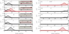
In Fig.  3, we present the probability-density profile of edge-state wave functions | ψ | ² as a function of the atom positions along the width of the graphene sheet for the six edge states labeled by A– F in Fig.  2. It is shown that states A and C are localized along the left edge, whereas B and D are localized along the right edge. Therefore, the edge states A  (B) and C  (D) have reversed chiralities and propagate in opposite directions along the left (right) edge, as shown in the inset of Fig.  3(a). Each of the two chiral edge modes carries an ± e²/2h conductance yielding total conductance G = 2e²/h. As M = Δ , the spin-up hole edge state (state E) and the spin-down electron edge state (state F) have the same velocities and are localized along the left and right edges propagating in the same direction, as shown in Figs.  2(b), 2(d) and 3(e), 3(f), resulting in a conductance G = e²/h. When M < Δ (the phase 1), the Fermi energy is located at the band gap of both two spin bands, and the charge and spin Hall conductivity are all zero (the conductance G = 0), while the valley Hall conductivity has a quantized value. In fact, the similar quantum states can also emerge in the graphene ribbon with armchair edge when the symmetries are broken, which has been investigated by many authors.^{[38– 42, 42]}

Fig.  3.

	Figure Option ViewDownloadNew Window
	Fig.  3. Probability density across the single-layer graphene sheet for the edge-state wave functions | ψ | 2 of the edge states labeled A– F in Fig.  2. The inset is a schematic diagram which indicates the propagation direction of the corresponding edge modes.

A lot of new quantum states with half integer conductance^[20] have been reported in experiment by applying a gate voltage, which indicates that the new quantum states with particular edge states properties may appear due to the variation of local potential by applying a gate voltage. In Fig.  4, we plot the phase diagram of quantum phases in graphene when the Fermi energy departs from the Dirac point. It is shown that the new quantum states with quantum number (− 1, ± 1, ± 1) emerge. At the phase boundaries, there are a lot of half integer quantum states, such as (− 1/2, − 3/2, 1/2) (the phase 4) and (− 1/2, − 1/2, 3/2) (the phase 6).

Fig.  4.

	Figure Option ViewDownloadNew Window
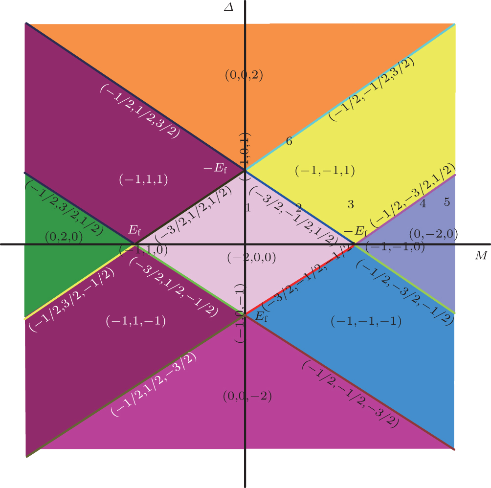	Fig.  4. Phase diagram in the M– Δ panel for the Fermi energy at Ef = − 0.05t. Heavy lines represent phase boundaries, which represents the points where the Fermi energy crosses the flat part of the energy band. A number shows a point where the energy spectrum is calculated and shown in Fig.  5.

Fig.  5.

Figure Option ViewDownloadNew Window

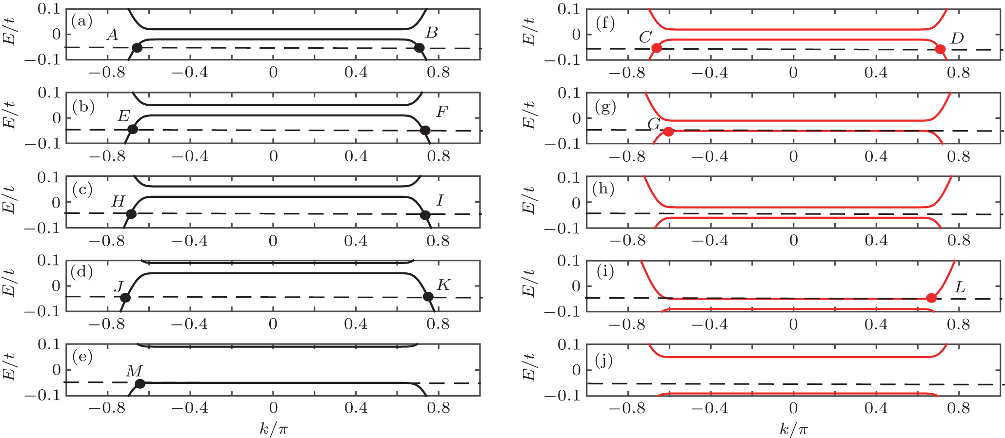Fig.  5. Edge-state band structure of the spin up (black lines) and spin down (red lines) of a zigzag graphene ribbon at marked points in the phase diagram shown in Fig.  4. Parameters are Δ = 0.02t and M = 0.0t in panels  (a) and (f) (the phase 1), M = 0.03t in panels  (b) and (g) (the phase 2), M = 0.04t in panels  (c) and (h) (the phase 3), M = 0.07t in panels  (d) and (i) (the phase 4), and M = 0.02t, Δ = 0.07t in panels  (e) and (j) (the phase 6).

The band structure and probability-density profile of the states labeled by 1∼ 6 in Fig.  4 are shown in Figs.  5 and 6. When M = 0 (the phase 1), the Fermi energy lies in both spinup and spin-down hole bands. The states A  (B) andC  (D) have the same velocities and propagate along the same + x  (− x) direction. It is shown in Figs.  6(a) and 6(e) that the states A  (B) and C  (D) are localized at the left (right) edge of graphene ribbon. Therefore, the states A  (B) and C  (D) propagate along the left (right) edge in the + x  (− x) direction, as shown in the inset of Fig.  6(a). As M increases, the spin-up band shifts upwards and the Fermi energy always lies in the hole band, so the states A  (B), E  (F), H  (I), J  (K), M always propagate along the + x  (− x) direction and localize at the left (right) edge, as shown in Figs.  5(a)– 5(e) and Fig.  6. However, for the spindown edge states, the case is entirely different because the Fermi energy shifts from the hole band to the electron band as M increases. When M = 0.03t (the phase 2), the Fermi energy crosses the flat part of the spin-down hole band, and the state G propagates along the left edge in the + x direction resulting in a G = 3e²/2h conductance, as shown in Fig.  5(g) and Fig.  6(b). As M = 0.04t the Fermi energy locates at the gap of the spin-down band (the phase 3), as shown in Fig.  5(h). The spin-up edge state flows along the two nanoribbon edges in opposite directions and contributes to the G = e²/h conductance. For the phase 5, it is the QSH phase and has the same property with the phase 3 in Fig.  1.

Fig.  6.

	Figure Option ViewDownloadNew Window
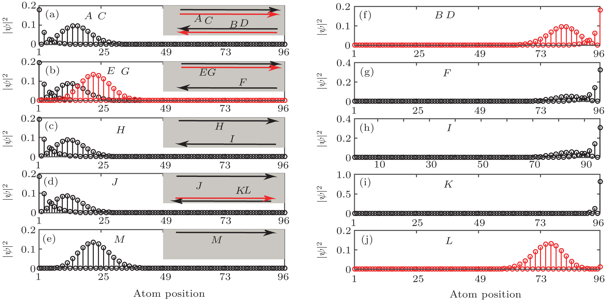	Fig.  6. Probability density across the single layer graphene sheet for the edge-state wave functions | ψ | 2 of the edge states labeled A– L in Fig.  5. The inset is a schematic plot which indicates the propagation direction of the corresponding edge modes.

In addition, there are two phases with e²/2h conductance (the phases 4 and 6), as shown in Fig.  4. For the phase 4, the Fermi energy crosses the flat part of the spin-down electron band, and the state L is localized at the right edge propagating in the opposite direction to the state K. However, for the phase 6 the Fermi energy crosses the flat part of the spin-up band and locates in the gap of the spin-down band, the state M propagates in x direction and is localized at the left edge.

We have investigated the possible quantum Hall states in graphene by considering an external magnetic field, the Zeeman spin splitting, and the sublattice potential. We have shown that at a large Zeeman energy, a quantum spin Hall phase appears with the helical edge states counter-propagating along the edges without spin– orbit interaction. As the Zeeman energy decreases, the QSVH phase emerges with one spinup edge state on one edge and one spin-down edge state on the other edge of the graphene flowing in the same direction, which leads to a unity conductance. At a weak Zeeman energy, the QVH phase appears with zero conductance. It is also found that at the phase boundary connecting the two different phases, new phases with half integer conductances in the experiment emerge when the Fermi energy deviates from the Dirac point.