† Corresponding author. E-mail:
A new reliable cellular automaon (CA) model designed to account for stochasticity in traffic flow induced by heterogeneity in driving behavior is presented. The proposed model differs from most existing CA models in that this new model focuses on describing traffic phenomena by coding into its rules the key idea that a vehicle’s moving state is directly determined by a driver stepping on the accelerator or on the brake (the vehicle’s acceleration). Acceleration obeys a deformed continuous distribution function when considering the heterogeneity in driving behavior and the safe distance, rather than equaling a fixed acceleration value with a probability, as is the rule in many existing CA models. Simulation results show that the new proposed model is capable of reproducing empirical findings in real traffic system. Moreover, this new model makes it possible to implement in-depth analysis of correlations between a vehicle’s state parameters.
To investigate dynamic traffic flow behavior on road segments in heavily populated cities, and to obtain a clear understanding of traffic phenomena, a number of models have been proposed. These models can be classified into macroscopic, mesoscopic, and microscopic models according to different scales of stepping mechanism. Macroscopic models, which mainly include fluid-dynamics models[1] and gas-kinetic-based models,[2] describe traffic in aggregated quantities. Microscopic models, which mainly include car-following models[3] and cellular automaton models,[4] focus on describing the status of each vehicle. At the intersection between macroscopic and microscopic models, the mesoscopic modelling applies principles of non-equilibrium statistical mechanics to kinetic theory to model the traffic flow.[5] For details on available traffic simulation methods and tools which can be used at various modelling levels, the reader can redirect to the work of Barceló.[6]
Cellular automaton (CA) model in traffic flow simulation was first proposed by Nagel and Schreckenberg in 1992. Four step updating rules were developed in NaSch model including acceleration, deceleration, random delay, and position update which laid a good foundation for reproducing the phenomenon of real traffic flow.[7] The classic NaSch model is however, limited in that it cannot reproduce some essential features of traffic flow such as phase separation and the hysteresis effect, etc.[8, 9] Kerner therefore proposed a three-phase theory of traffic,[10] which divides congested traffic into two phases: synchronized flow and wide moving jams. Many models based on Kerner’s theory followed,[11–16] and were able to successfully reproduce the fundamental diagram of traffic and the spatiotemporal shapes of the different traffic phases. Moreover, there are many studies on traffic flow behavior in different scenarios based on CA models,[17–22] which all prove that CA models are able to provide considerable insight into traffic behavior and are very promising alternatives to modeling traffic flow and understanding its behavior despite that different models usually have different advantages and disadvantages.[23]
The biggest common advantage of CA models is local rule-based mechanism, which means that vehicles make decisions based on their goals, their current situation, and interactions with their surroundings. This peculiarity ensures that CA models are able to capture micro-level dynamics.[24] However, there is a disadvantage of CA models in micro-level step updating mechanism which received little attention in the last decades when we look into models’ micro-level dynamics. Most existing CA models include the rule that vehicles adjust their velocity directly according to the headway distance and take into consideration the stochasticity in traffic flow by introducing a certain probability in control of changes in vehicles’ velocity.[25–27] Consequently, vehicles tend to change speed abruptly, exceeding the real vehicular acceleration/deceleration capabilities and producing erratic acceleration/deceleration behavior.[28] Some CA models introduce limited acceleration/deceleration capability into the CA traffic flow model[29] and set the acceleration and deceleration rates to be specific constants with a certain probability according to the traffic condition. This setting is able to overcome the erratic acceleration/deceleration problem. However, these models are still unrealistic since it is known, from many observed trajectories in real traffic, that different accelerations/decelerations induced by heterogeneity in driving behavior usually are continuously distributed random variables and are highly related to safe distance[30] and relative velocity between adjacent vehicles.[31, 32] In brief, despite plentiful research on CA modelling application, insufficient attention has been paid to improving models’ fundamental micro-level step updating mechanism coupling with the consideration of safe distance and relative velocity between adjacent vehicles. This motivated the writing of this paper.
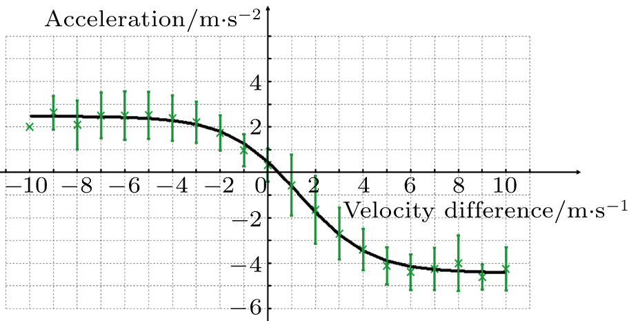
In this paper, a new CA model accounting for stochasticity in traffic flow induced by heterogeneity in driving behavior is proposed for traffic flow, which is both simple and reliable. Our model also introduces the concept of safe distances to give a more reasonable upper limit to acceleration of vehicles. The two main new features introduced are: (i) A vehicle’s moving state is directly determined by a driver’s action of accelerating or braking (acceleration of a vehicle), rather than assuming velocity is directly determined by the headway distance; (ii) The acceleration rate in this model obeys a deformed continuous distribution function according to the annual research report prepared for the U.S. Department of Transportation.[33] These new features make our proposed model more realistic in traffic flow simulation.
The remainder of this paper is organized as follows. Section
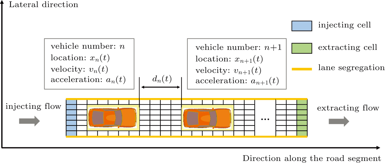
The new proposed model is defined on a lattice of length L, where each cell can be empty or occupied by just one vehicle. The system consists of N vehicles moving in one direction in a single lane, therefore overtaking and lane changing are not permitted. The speed of each vehicle can take on one of the (V
max+1) allowed integer values 


A definition of safe distance d
safe is introduced before considering the micro-level step updating mechanism of the model. Suppose there are N vehicles in total, denoted by 

 |


 |

 |


According to many previous studies, if a driver decides to accelerate or decelerate they prefer to use the comfortable acceleration 

If 
 |
 |
In the above equation, the terms 


The value of acceleration should be a discrete integer in CA models. Thus, the probability of acceleration, 


 |
One update of the system consists of the following consecutive steps.


 |
 |


The simulation scenario used for the simulation study is described below. We assume that private cars are the only vehicle type for the simulation. According to a previous study, it is plausible to assume that these moving vehicles occupy 5 × 5 cells if the size of one cell is 1 m 

The speed limit on urban roads in China is 70.00 km/h when there is only one lane in each direction. For this study, the maximum velocity is set to be 


Simulation results for a single-lane road segment with periodic boundary conditions are shown here. The injecting cells and the extracting cells are coincident in the periodic boundary conditions. The global density ρ is defined as
 |
 |

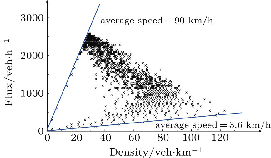
Initially, the vehicles stop near the injecting cells in a line and then start up one by one based on the proposed model. In order to get to a stable state of the system, each simulation, with different values for density ρ, is conducted for 3.6×10³ time steps after a spin-up period of the first 103 time steps. Flow, velocity, and density are the commonly used parameters which represent the most important macroscopic traffic characteristics.[38] If the flow is measured in “vehicles/h”, the relationship between density ρ and flow q, and the correlation between vehicles’ average velocity and density ρ are shown in Fig.
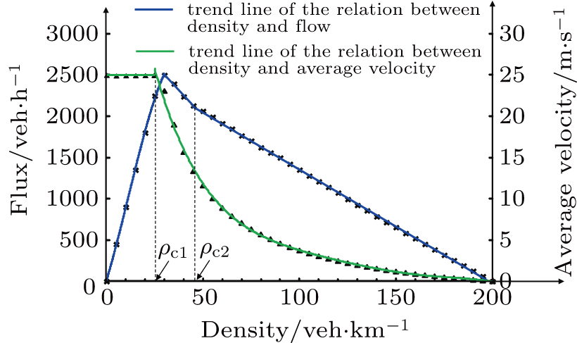 | Fig 2. The fundamental diagram and the correlation between density and velocity of the proposed model. |
The density–flow relationship and the density–velocity relationship obtained from the simulations of this model are consistent with the classical and empirical findings obtained in some other prevalent models such as the BJH model,[37] the Slow-to-start model,[39] and the comfortable driving (CD) model.[40] Our proposed model is also able to reproduce the hysteresis phenomenon and the three phases (free flow, synchronized flow, and jammed flow) observed in real traffic, as is shown in Fig. 


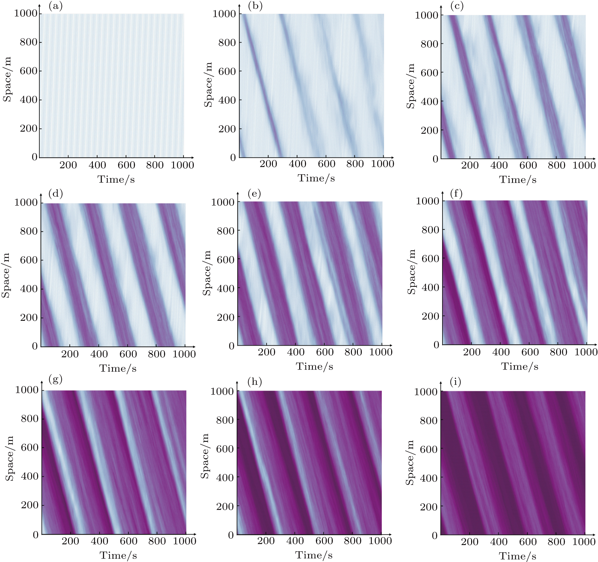
The spatiotemporal shapes of different traffic phases (free flow, synchronized flow, and jammed flow) for different simulation scenarios are depicted in Fig.
From Fig.
To depict the three traffic states (free flow, synchronized flow, and jammed flow) more clearly, Figure 

 |
The most important difference between Fig.
We also find that the performance of this proposed model is more realistic by analyzing the correlations between one vehicle’s different state parameters. A series correlation analysis of a vehicle’s state parameters was conducted to illustrate the performance of the proposed model in a more detailed way.
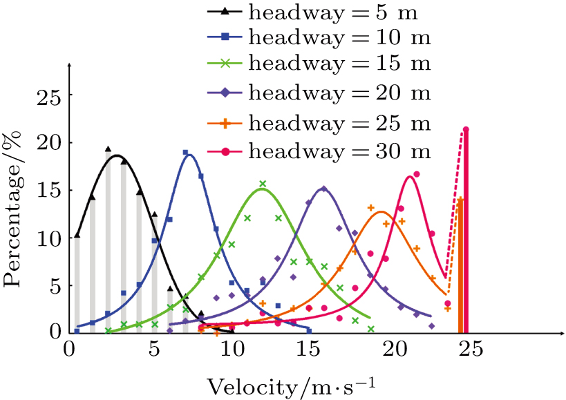
The distributions of the velocity with different headway distances are shown in Fig. 
The distribution becomes approximately symmetrical and the axis of symmetry moves gradually in the positive direction along the “velocity” axis, together with headway distance increasing (headway=10 m, 15 m, 20 m). When the headway distance is 25 m or 30 m, the velocity distributions become asymmetrical again and present distributions with two peaks. The second peak is at “velocity=25 m/s”. The second peak becomes bigger with increasing headway distances which means that with a bigger headway distance, more vehicles can move ahead with maximum velocity.
We use nonlinear curve fitting in OriginPro 9.1 to fit the obtained data scatter points. In general, the distribution curves (without the second peak if it exists) fit a Lorentz distribution well in a discrete state with the following probability density function
 |
| Table 1.
The values and standard errors of the parameters in Eq. ( |
From Table
 |
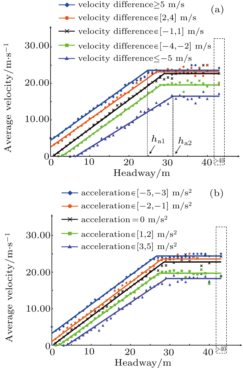 | Fig 6. The correlation between the headway distance in front of a vehicle and the average velocity of that vehicle. |
We next study the correlation between the headway distance and the average velocity with the simulation results grouped according to the acceleration of vehicles. The corresponding results are shown in Fig.
From Fig.
Suppose that 


 |
 |
 |
 |


The fitting equation in Fig.
 |
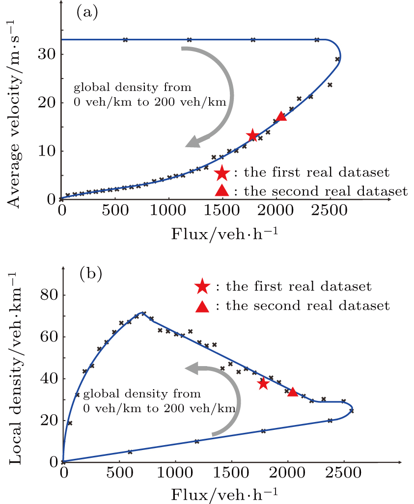
We use data extracted from real traffic flow by other researchers to verify our proposed model from both macroscopic and microscopic perspectives, as shown in Table
| Table 2.
Two datasets extracted from real traffic flow. . |
The first dataset was derived from empirical video data on the Nanjing Airport Highway.[45] This highway is the main road connecting Nanjing urban areas with Nanjing Lukou Airport. There were 40 cameras along the 28-km-long highway which has two lanes in each direction. The second dataset was obtained from a large-scale construction project also situated on the Nanjing Airport Highway. Every day one of the two lanes was temporarily closed on a 5–10-km-long section of road. This enabled the collection of empirical single-lane traffic flow data.[46, 47] The speed limit in both traffic scenarios was 120 km/h (
We adjusted the maximum velocity in our proposed model from 25 m/s to 33 m/s to make the simulation conditions same as real traffic scenarios in datasets. A virtual detector was set at the end of the road. Each simulation, using a certain global density lasted for one minute, and sixty groups of simulations with the same global density were conducted. The sum of the fluxes from these sixty groups and the average velocity of the vehicles that passed by the virtual detector were recorded. Then the local densities for different fluxes were calculated using 
The above validation proves that the proposed model is a competitive CA model. The proposed model can simulate traffic flow ensuring the authenticity of the features, and is able to reproduce the empirical findings. Moreover, we found that the acceleration of a vehicle is mostly influenced by the velocity difference when the absolute value of acceleration is not large. This finding is consistent with other studies which showed that acceleration always has a linear correlation to the velocity difference when the absolute value of acceleration is not large.[31, 32]
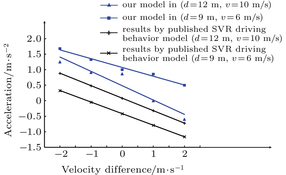
We compare the results produced by our proposed model with those produced by the SVR driving behavior model. Wei and Liu depicted the correlation between relative velocity and acceleration for headway distances of 9 m and 12 m.[31] The relative velocity is in an interval of [–10, 10] km/h ([–2.78, 2.78] m/s). We therefore analyzed the coupled distribution of velocity and velocity difference in a case study using our proposed model for headway distances of 9 m and 12 m. The results are shown in Table
| Table 3.
Coupled distribution (%) of velocity and velocity difference with headway distance of 9 m. . |
| Table 4.
Coupled distribution (%) of velocity and velocity difference with headway distance of 12 m. . |
Since, in the proposed model, 


The values of acceleration are a little higher than the results of the SVR driving behavior model, mainly because this model’s acceleration strategy of allowing a driver to accelerate as long as there is a safe headway distance, is more radical than that of the SVR driving behavior model. The results also show that the proposed model reveals the law that acceleration has a linear correlation with the velocity difference when the absolute value of acceleration is not, in general, large. Thus, the results reflect the superiority of the proposed model, in that this model can present more detailed correlations between state parameters. The results indicate that the assumption that acceleration and deceleration rates can be considered to be constant in most empirical models, needs to be reevaluated.
In this paper, we describe and then analyze a new cellular automaton (CA) model designed to account for stochasticity in traffic flow induced by heterogeneity in driving behavior. The proposed model overcomes two major limitations of many of the published CA models for traffic modeling. One is the overdependence on directly changing a vehicle’s velocity in the model’s updating rules, and the other is the selection of a discrete constant value for acceleration which does not completely accord with reality. The proposed model also takes into account using safe distances to limit the value of acceleration to avoid collisions between vehicles. The model still uses discrete integer values for the state parameters of vehicles in the model simulation. As is well known, the calculation and execution time of a CA model is proportional to both the number of vehicles in the system and the number of iteration steps. The calculating and executing efficiency of the proposed model is 

Simulation results indicated that the new model is a highly capable model for modeling traffic flow whose performance is quite competitive from both macroscopic and microscopic perspectives. In particular, simulation results for a road segment with periodic boundary conditions indicated that the proposed model is capable of reproducing most empirical findings, including the fundamental diagram which depicts the three phases (free flow, synchronized flow, and jammed flow), and the backward movement of a traffic jam in congested flow. This model also has a stronger ability to simulate free flow, light synchronized flow, and heavy synchronized flow at the same time.
This model can also take apart the detailed coupling correlation between a vehicle’s different state parameters, which is difficult for other existing CA models. This model is capable of delineating the distributions of velocity with different headway distances, the correlation between the headway distance and the average velocity, and the correlation between velocity difference and acceleration of vehicles. The proposed CA model also shows that acceleration has a linear correlation with velocity difference when the absolute value of acceleration is not particularly large in general which is consistent with common findings in other models.
We plan to extend our proposed model in future to incorporate more realistic urban traffic systems, taking into consideration different types of vehicles and real-time updates of traffic conditions.
| [1] | |
| [2] | |
| [3] | |
| [4] | |
| [5] | |
| [6] | |
| [7] | |
| [8] | |
| [9] | |
| [10] | |
| [11] | |
| [12] | |
| [13] | |
| [14] | |
| [15] | |
| [16] | |
| [17] | |
| [18] | |
| [19] | |
| [20] | |
| [21] | |
| [22] | |
| [23] | |
| [24] | |
| [25] | |
| [26] | |
| [27] | |
| [28] | |
| [29] | |
| [30] | |
| [31] | |
| [32] | |
| [33] | |
| [34] | |
| [35] | |
| [36] | |
| [37] | |
| [38] | |
| [39] | |
| [40] | |
| [41] | |
| [42] | |
| [43] | |
| [44] | |
| [45] | |
| [46] | |
| [47] |


