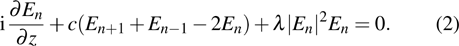
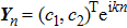
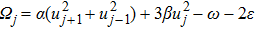
1. IntroductionAs is well known, discrete soliton appears in a wide variety of physical areas, e.g., atomic chain[1,2] with on-site cubic nonlinearities, electrical lattices,[3] biophysics,[4,5] and in arrays of coupled nonlinear optical wave guides.[6,7] It has been demonstrated that a discrete nonlinear Schrödinger (dNLS) equation, integrable or nonintegrable, can be used as the models describing the discrete phenomena in the real physics. The dNLS describing the electric field propagating in nonlinear optical waveguide arrays was first introduced by Christodoulides and Joseph.[8] By using the formalism of coupled-mode theory and considering only nearest-neighbor interaction, they showed that the electric field propagating in the nonlinear optical waveguide obeys
where the nonlinear term

describes the self-phase modulation that takes place in the
nth waveguide, and the term
arises from the nonlinear overlap of the adjacent modes. It is difficult to study the discrete model (
1). However, in many cases, the self-phase-modulation term

dominates the nonlinear process. Hence, they set
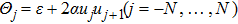
μ = 0, and discussed the nonintergable discrete NLS
The nonintergable dNLS also has applications in biophysics for explaining some of the fundamental questions, such as transfer, storage, and movement of vibrational energy in polypeptides.
[4] The dNLS equation (
2) has been investigated in terms of many aspects, including Hamiltonian analysis,
[5] dynamics behaviors,
[9–13] and discrete perturbation.
[14] By using discrete Fourier transformation, Ablowitz and Musslimani constructed stationary and travelling soliton waves of dNLS equation (Eq. (
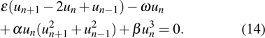
2)).
[14] However, as is well known, if we neglect the nonlinear nearest-neighbor interaction term, much important information, e.g., the shape of the wave, for the electric field propagating in nonlinear optical waveguide arrays, might be missed.
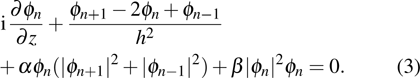
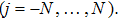
In this paper, we study the discrete model (1) which can be rewritten as
We emphasize here that the nonintegrable dNLS equation (
3) cannot be obtained by the reduction of Eq. (
4) in Ref. [
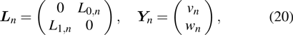
15]. The modulation stability of nonlinear plane-wave solutions of Eq. (
3) is discussed.
[16] By using discrete Fourier transformation, we will give numerical solitary waves for the two cases of stationary and traveling types, respectively. The stability analysis of stationary solitary waves will be discussed. It is shown that the nonlinear hopping term has great influence on the form of solitary wave. The shape of solitary wave is the important information in the electric field propagating. We will demonstrate that the solitary wave possesses new behaviors, e.g., in the defocusing case, i.e.,

, and there exists the discrete bright soliton. This quite contradicts the discrete integrable case, or the ones of continuous integrable systems. Furthermore, we also test the effectiveness of the nonintegrable NLS equation (
3) as a discrete model for the NLS equation. Numerical simulation shows that the discrete model (
3) is better than the model (
2).
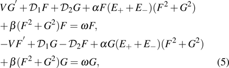
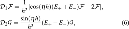
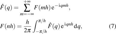
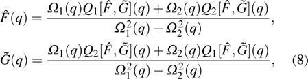
2. Stationary and traveling solitary waves from discrete Fourier transformationIn this section, by using the discrete Fourier transformation approach,[14] we will obtain numerical approximations of discrete localized stationary and traveling solitary waves for nonintegrable dNLS equation (3). The key point of the method is to transform a differential advance-delay equation into a nonlinear integral equation which can be solved numerically. The stability of stationary solitary waves will be conducted. We should remark here that though there is a standard method based on the solution of the nonlinear eigenvalue problem to find localized solutions of discrete systems (see e.g., Ref. [17]), in order to compare with the corresponding results of nonintegrable discrete NLS equation (2), we employ the discrete Fourier transformation approach to deal with Eq. (3).
2.1. Transform a differential advance-delay equation into a nonlinear integral equationSetting ϕn in the form
where
ξ =
nh−
Vz,
, and
, with
V and
ω being the soliton velocity and wave-number shift, respectively, equation (
3) is reduced to the following differential advance-delay equation:
where prime denotes the derivative with respect to
ξ and
with
. It is very difficult to find a solution to the system (
5). To solve Eq. (
5), we employ the discrete Fourier transformation. Introducing the discrete Fourier transform,
then the system (
5) can be transformed into the nonlinear integral equations as follows:
where

and,
with
It should be remarked that when we derive Eq. (
8), we have used the following discrete Fourier transformation for
F(
ξ),
ξ =
nh−
Vz, and its property
Furthermore, in order to obtain a solution for the integral equation (
8), we will employ the Petviashvili method, or modified Neumann iteration scheme.
[17–20] 2.2. Stationary solitary waveTo obtain discrete localized stationary solitary wave, we set V = 0, η = 0,
 , and G = 0. Then system (8) is reduced to the following nonlinear integral equation:
where
is the frequency of the linear excitations. We construct function sequences

defined by
Numerical simulation shows that by choosing the proper values for the parameters, then as

and the function sequence

is convergent. We set

as

. Then

is a fixed point of nonlinear integrable equation (
11), and its inverse Fourier transformation
F(
nh) is an approximate solution of nonintegrable dNLS equation (
3).
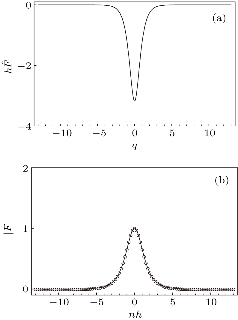
Let us give a numerical example with the parameters and initial value being: α = 2, β = 1, ωs = 1,
 . The result of the numerical simulation is given in Table 1.
In the following numerical examples, we take the values of the parameters which include three cases of
 ,
,
 , and α + β = 0. They correspond respectively to focusing NLS, defocusing NLS, and LS equations.
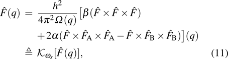
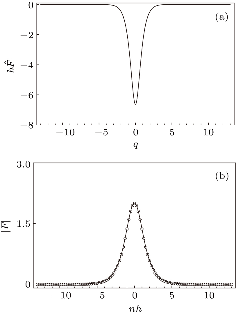
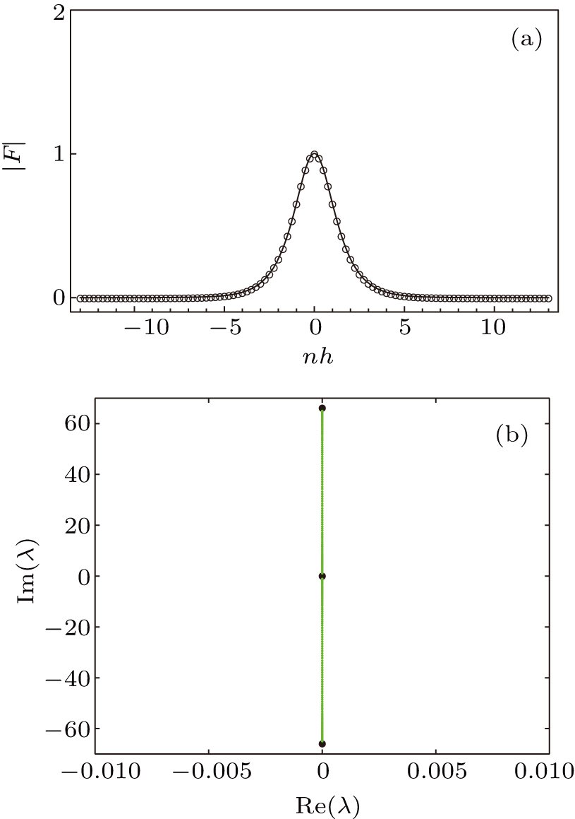
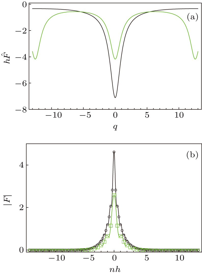
Figure 1 gives the shapes of the stationary solitary wave with the different nonlinear nearest-neighbor interaction term parameter α in Fourier domain and physical space, where the nonintegrable term β, wave-number shift ωs, and the lattice spacing h are fixed. We find that the nonlinear nearest-neighbor interaction term parameter α has influence on the solitonʼs amplitude. When the nonlinear term parameter α = −0.5, the amplitude of the soliton attains the maximum. When α increases from −0.5 and α decreases from −0.5, the amplitude decreases monotonically in both two cases.
This type of solution is called discrete breathers.[21,22]
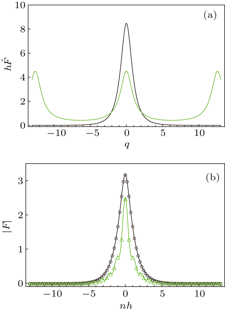
Figure 2 describes an oscillate solitary wave, where ωs = 1, β = −1, α = 0.5 (2α + β = 0), with two different values of lattice spacing, h = 0.25, and h = 0.5.
Figure 3 gives a discrete bright soliton, where we choose parameters ωs = 1 and h = 0.25, α = 0.5, β = −0.5
 . However, under the situation
 and
and
 , we can also obtain the bright soliton, which is shown in Fig. 4, where the parameters ωs = 1, β = −1, and h = 0.25, α = −0.5
 . This result contradicts with the ones in the discrete integrable cases or the ones of continuous integrable systems.
Figure 5 shows an oscillate solitary wave in the case of
 . We can see that the structures of solitary waves for nonintegrable discrete NLS equation (3) with the nonlinear nearest-neighbor interaction are much more richer than those of solitary waves for nonintegrable discrete NLS equation (2) without the term. As is well known, the shape of solitary wave is the important information in the study of the electric field propagating. When we use the nonintegrable discrete NLS equation (3) with the nonlinear nearest-neighbor interaction as the model of electric field propagating, we can modulate the shape of the wave by choosing the self-phase modulation and the term of the nonlinear overlap of the adjacent modes.
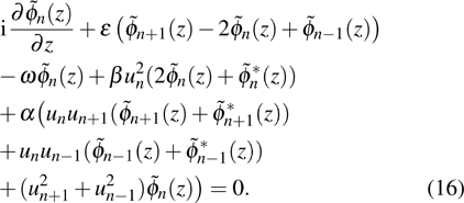
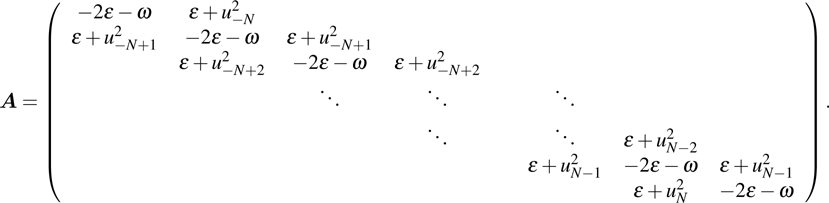
2.3. Analysis of linear stability for stationary solitary waveIn this subsection, following the idea in Ref. [23], we examine the linear stability of stationary solutions of the nonintegrable discrete NLS equation (3). For convenience, we set ε = 1/h2. We have known that the nonintegrable discrete NLS equation (3) admits the following localized stationary solution:
where
un is a localized real function (i.e.,

as

) and satisfies the difference equation
To study the linear stability of solution (
13), we consider the behavior of the stationary solution under small perturbations. Inserting the perturbed solution
into Eq. (
3) and dropping the terms of quadratic and higher order in

, we derive a linear equation with respect to

,
By substituting the solution in the form of normal modes with the eigenvalue
λ
into Eq. (
16), and introducing the variable transformation
we obtain the discrete linear eigenvalue problem
where
and
There exists a continuous spectrum as

with the eigenfunction

given by
, where
k is a real wavenumber,

are constants. Solving Eq. (
19) gives the continuous eigenvalues
. Thus the continuous spectrum of Eq. (
19) extends over the intervals [
ω,
ω + 4
ε] and [−(
ω + 4
ε),−
ω] on the imaginary axis.
Note that λ = 0 is a discrete eigenvalue which has a discrete eigenfunction
 and a generalized discrete eigenfunction
 ,
,
We remark here that the so-called generalized discrete eigenfunction refers to the relation:

.
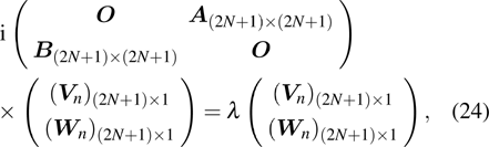
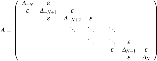
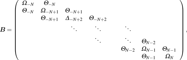
To look for the nonzero discrete eigenvalue of Eq. (19) through the numerical method, we truncate the lattice n to
 , then the infinite-dimensional discrete eigenvalue problem (19) reduces to the case of the finite-dimensional one
where

,

,

, and

are, respectively
with
with
,
.
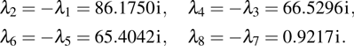
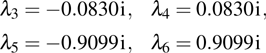
Let us give out the discrete spectrum of the different stationary solitary waves corresponding to the cases of Figs. 1–5. As described in Ref. [23], a necessary condition for the stability of stationary solitary waves is that
 for all eigenvalues. A sufficient condition for the instability is that at least a discrete eigenvalue λ, s.t.,
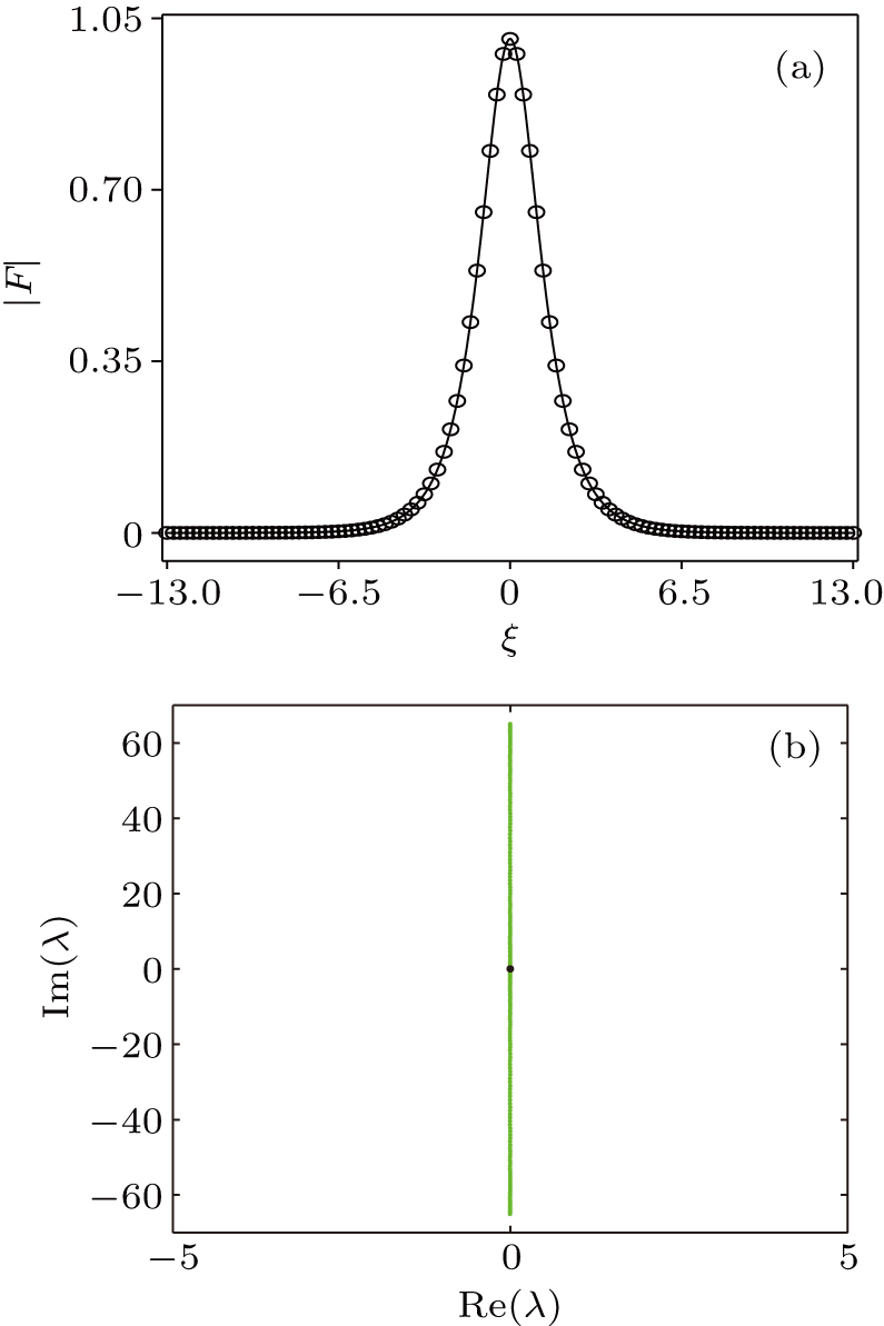
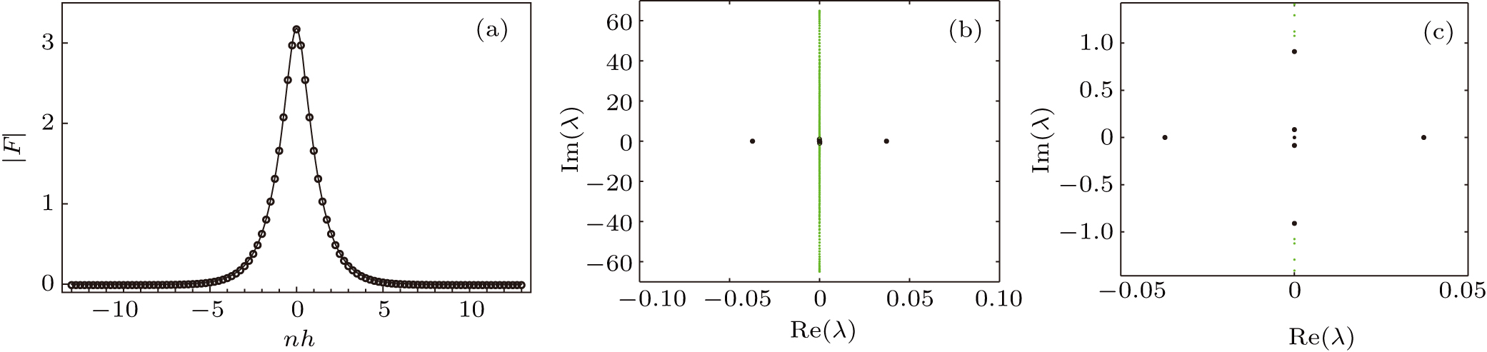
 . Considering the accuracy of numerical simulation, we set h = 0.25. Then taking ω = 1 yields the intervals i[1,65] and i[−65,−1] for the continuous spectrum which is described by the green line in the figures. We choose N = 52 in Figs. 6–11.
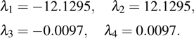
For the stationary solitary wave in Fig. 6(a) with 2α + β = 0,
 , the discrete spectrum of the linearization operator Ln contains two pairs of real eigenvalues in Figs. 6(b) and 6(c). The real eigenvalues are
Since there exist two positive real eigenvalues, the corresponding perturbed solution will exponentially grow with
z, i.e., the stationary solitary wave in Fig.
6(a) is linearly unstable.
For the stationary solitary wave in Fig. 7(a) 2α + β = 0,
 , four pairs of discrete eigenvalues are located at the imaginary axis, which are called internal modes. They are
In this case, the perturbed term

will oscillate with
z.
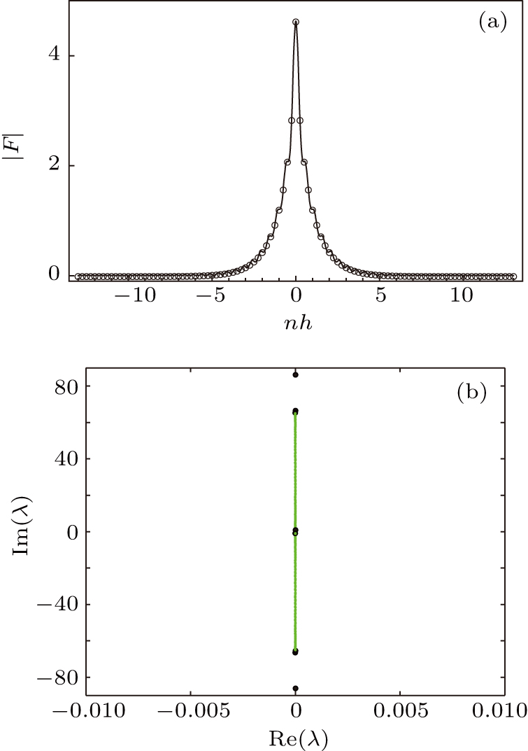
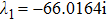
A pair of real eigenvalues and three pairs of internal modes for the stationary solitary wave in Fig. 8(a) with
 ,
,
 are given in Fig. 8(b). The real eigenvalues are λ1 = −0.0208 and λ2 = 0.0208. Three pairs of internal modes are
The positive real eigenvalue leads to the linear instability of the solitary wave in Fig.
8(a).
A pair of internal modes
 and
and
 appear in Fig. 9(b) as the parameters are ωs = 1, α = −0.5, β = −1, h = 0.25. Like the case in Fig. 7(b), this indicates that the perturbed term
 will also oscillate with z.
For the stationary solitary wave in Fig. 10(a) with parameters ωs = 1, α = −0.4, β = 1, h = 0.25 (
 ,
,
 ), a pair of real eigenvalues λ1 = −0.0373, λ2 = 0.0373, and two pairs of internal modes
are obtained, see Figs.
10(b) and
10(c). Due to the occurrence of the positive real eigenvalue
λ2, this stationary solution is linearly unstable.
To compare with the linear stability of stationary solution (13) for nonintegrable discrete NLS equation (3) and an integrable discrete NLS equation
we investigate the linear stability of the stationary solution of Eq. (
25). The localized real function
un in stationary solution (
13) satisfies the following difference equation:
Under the action of the perturbed solution (
15), the corresponding operators for discrete linear eigenvalue problem (
19) is
Thus, the reduced finite-dimensional discrete eigenvalue problem (
24) becomes
where the matrix

is
The linearization operator Ln of the stationary solitary wave has only zero discrete eigenvalue except the continuous spectrum (see Fig. 11(b)). It should be remarked that as mentioned in Ref. [17], the appearance of nonzero discrete eigenvalues in the linearization spectrum of solitary waves is an important phenomenon of nonintegrable equations.
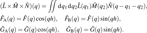
2.4. Traveling solitary wavesTo find the traveling solitary wave of the dNLS equation (3), we take the following iteration scheme:
where
Similarly, by numerical simulation, as

, we have
and function sequences

and

are convergent. We set

and
as

. Then

is a fixed point of nonlinear integrable equation (
8), and their inverse Fourier transformation

is an approximate solution of Eq. (
5).
Let us give two examples of numerical simulations for nonlinear integral equation (30).
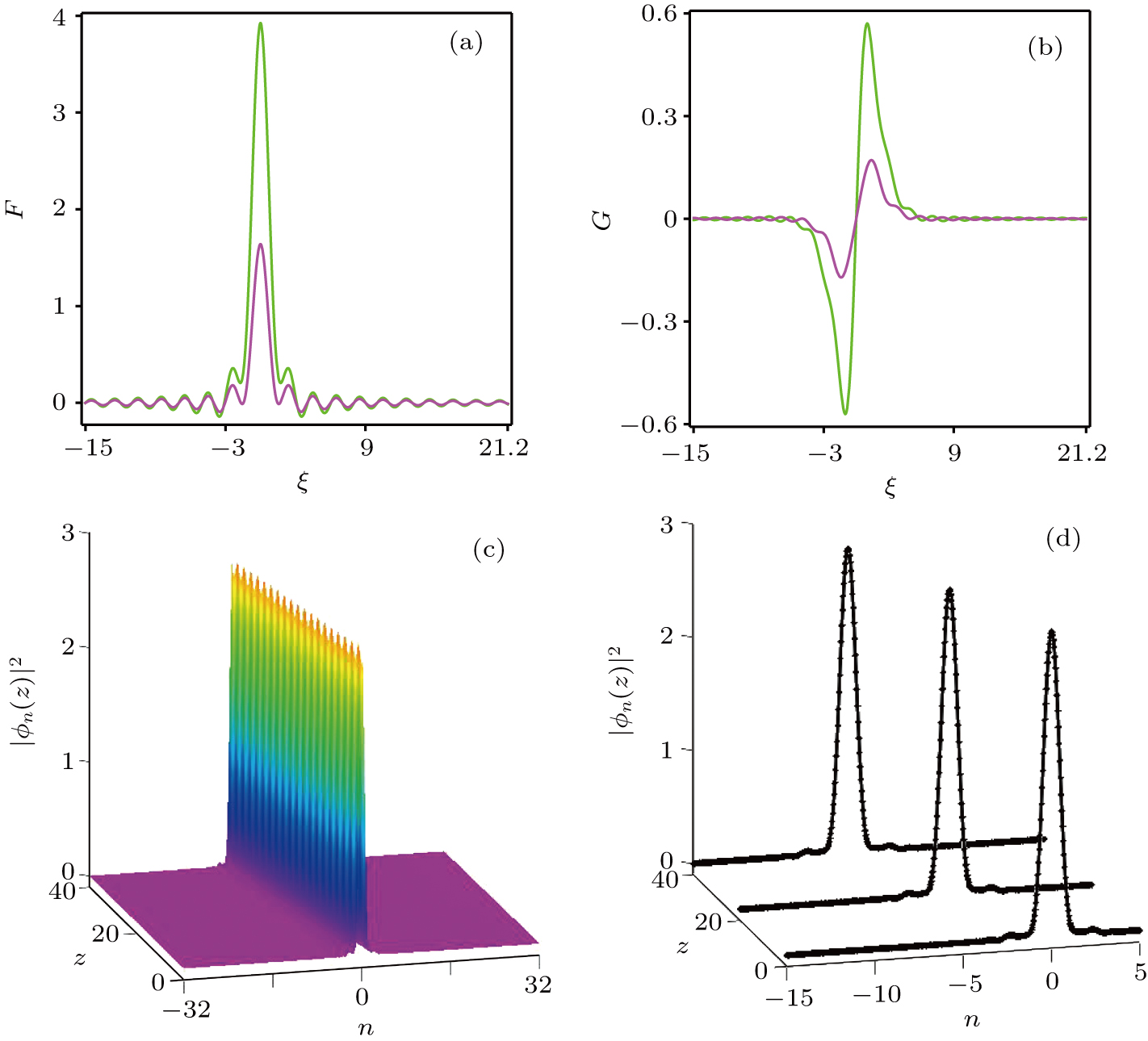
In this case, a typical traveling soliton solution to Eq. (3) is presented in Fig. 12. In Figs. 12(a) and 12(b), we can observe that the change of the parameter α has an influence on the amplitude of the soliton mode. Figure 12(c) describes a wave, which travels to the left. The hopping term has much more influence on the traveling solitons when
 approaches zero. Figure 13 displays the hopping property in the traveling soliton mode. From Fig. 13(d), we see that the amplitude of the soliton has some slight oscillations at the two sides of the wave. Similar results with stationary cases are obtained when
 is near zero. The modes of the traveling solitons have oscillations when
 is in a small neighborhood of zero.
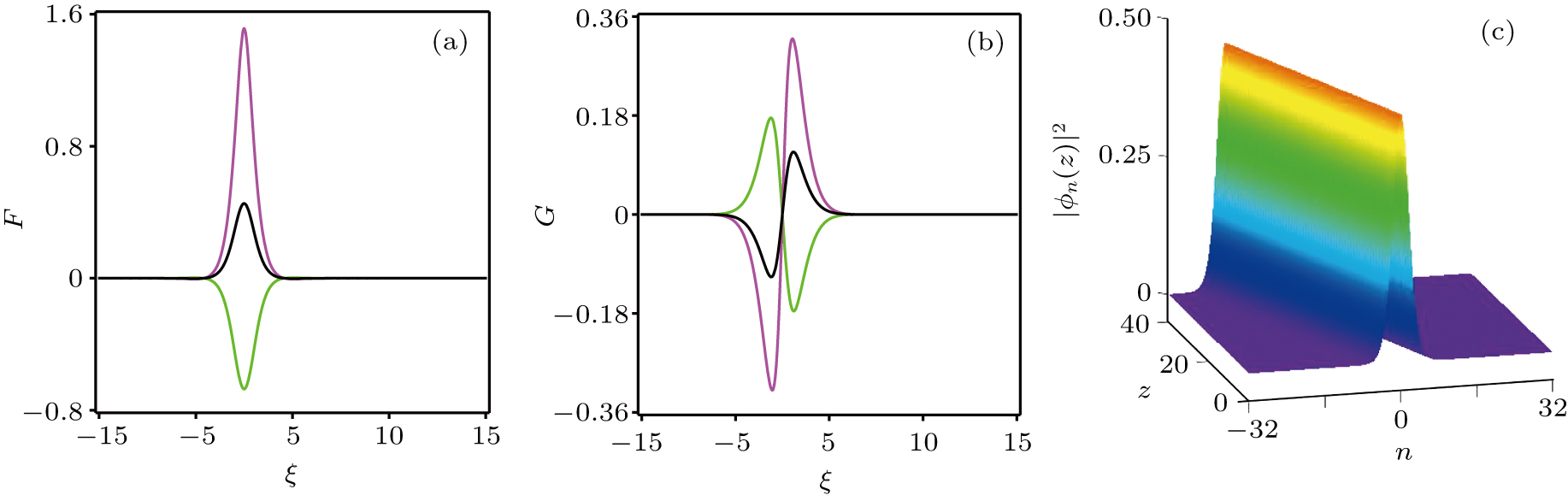
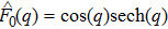
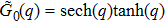
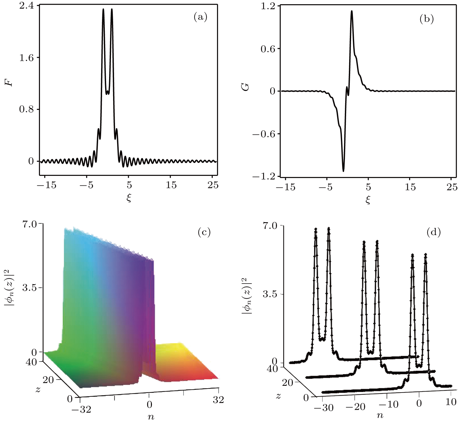
Figure 144(a) and 14(b) give the shapes of F(ξ) and G(ξ). Figure 14(c) and 14(d) describe the evolution of the traveling soliton. The traveling soliton possesses new behaviors, e.g., it has two peaks in the shape, and the oscillations occur not only at the edges of the wave, but also in the middle of the wave.
3. Chaos phenomenon between the nonintegrable dNLS equation with the term of nonlinear nearest-neighbor interaction and another nonintegrable dNLS equation without the termIn this section, we will show a difference of chaos phenomenon between the nonintegrable dNLS equation with the term of nonlinear nearest-neighbor interaction and another nonintegrable dNLS equation without the term. Herbst and Ablowitz[24] considered the Cauchy problem for NLS,
with periodic boundary condition
, and the initial condition
and

. They gave a numerical computation for the Cauchy problem. They proposed integrable discrete scheme (
25) of NLS and the following nonintegrable discrete scheme:
with the periodic boundary conditions

and
h =
L/
N. It has been demonstrated that the nonintegrable discrete scheme produces a chaotic solution for intermediate levels of mesh refinement, e.g.,
N = 32. However, chaos disappears when the discretization is fine enough, e.g.,
N = 50, and the convergence to a quasiperiodic solution is obtained. Numerical simulation has been performed by choosing
γ = 4,

,

(see Ref. [
24]). Here, we would like to test what happens if the discrete model is a nonintegrable discrete NLS equation (
3). Let us change Eq. (
3) into the following form:
where
α +
β = 1. Our numerical simulation (time integration is performed by the Runge–Kutta–Merson method) shows that model (
34) is better than the discrete model (
33), i.e., model (
2). In fact, by numerical simulation, we find that the nonintegrable discrete scheme (
34) still produces a chaotic solution for intermediate levels of mesh refinement. However, due to the integrable term

, the chaotic solution evolves gradually to a quasiperiodic solution with the integrable term increasing. For example, when
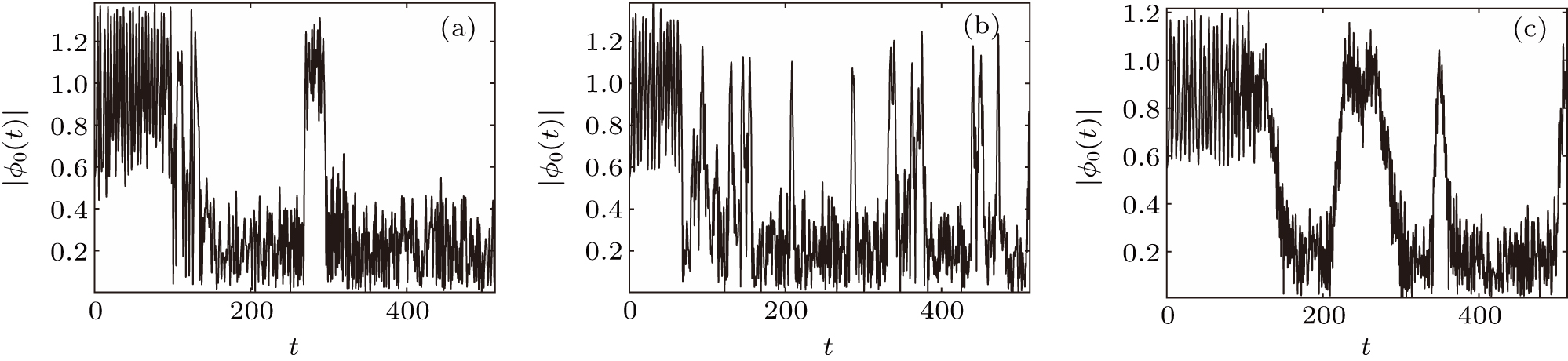
N = 8, from Fig.
15, we can see that the chaotic solution occurs. However, chaotic impact decreases with the term
gradually increasing. Furthermore, when mesh is refined to be
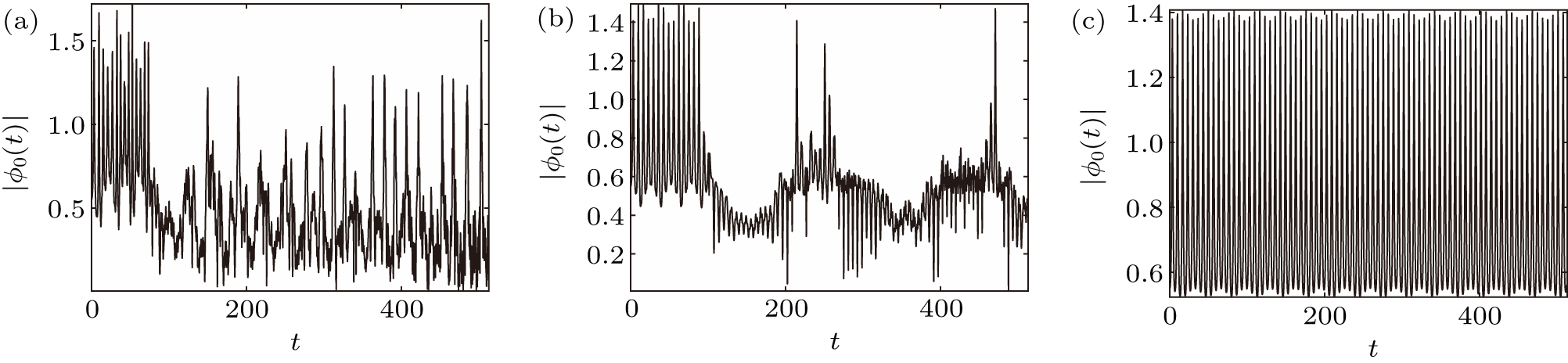
N = 32, if we choose
α = 0, or
α = 1/5,
β = 4/5, chaotic solutions still exist. However, if we choose
α = 1/3 and
β = 2/3, the chaos disappears and the solution evolves in a quasiperiodic way (see Fig.
16). This implies that the existence of chaos relates closely to the level of mesh refinement and the discrete model. The term of nonlinear nearest-neighbor interaction has significant influence on the disappearance of the chaos. We thus think that the discrete NLS model (
34) is better than the discrete NLS model (
33) in the sense that the convergence to a quasiperiodic solution for the Cauchy problem of NLS needs less number of grid points
N. We should emphasize again that nonintegrable discrete model (
34) has a solitary wave solution, and yields a chaos phenomenon for the Cauchy problem of the NLS equation. The chaotic solution evolves gradually to the quasiperiodic solution with integrable term increasing. If
β = 0, the model (
34) is integrable. Using the integrable scheme, a chaos phenomenon for the Cauchy problem of the NLS equation does not occur.


