The principle of Bell–Bloom magnetometer (BBM) is based on the discovery of Bell and Bloom in 1961, that the precession of atomic ground state polarization at Larmor frequency can be induced by synchronous amplitude-modulation (AM) of the optical pumping light with either circular^[1] or linear^[2] polarization. This technology was soon used in magnetometry and various versions of the BBM have been developed,^[3–7] including frequency-^[8,9] and polarization-modulation.^[10–12]

The precession of the atomic polarization can be measured by transmission of circular polarized light as well as nonlinear magneto-optical rotation (paramagnetic Faraday rotation) of linearly polarized light.^[13] Very high signal-to-noise ratio can be achieved by phase-sensitive detection referenced to the 1st or higher harmonics of the modulation frequency. It is often practical and convenient to pump and probe with a single beam. However, two-beam scheme has the advantage of allowing the separate study and optimization of the pumping and probing processes.^[14] Pustelny et al. studied AM BBM using a single linearly polarized beam for different light intensities, duty cycles and modulation wave forms.^[15] Schultze et al. compared the characteristics and performance of the M–x magnetometer with those of the AM BBM for different duty cycles and modulation depths.^[16] Grujic and Weis modeled and partially verified the magnetic resonance signals occurring in amplitude-, frequency-, and polarization-modulated light for the single-beam scheme.^[17] In those studies the pumping rate was much smaller than the transverse relaxation rate in the dark Γ₂ and power broadening was neglected. Compared with sinusoidal AM whose pumping-rate effect was well studied,^[18] square-wave AM has an extra control parameter, the duty cycle, allowing further tweaking the performance of the magnetometer. In this article we theoretically and experimentally analyze the effects of the pumping rate and the modulation duty cycle on the field response and the noise of the system. While most previous studies used pumping rates smaller than or comparable to Γ₂ and duty cycles on the order of several tens of percent, our study covers a range of duty cycles and corresponding pumping rates over 2 orders of magnitude. We find that, using a small duty cycle while keeping the time averaged pumping rate close to Γ₂, we can increase the field response of magnetometer at resonance by up to a factor of π/2 comparing to the common case of 50% duty cycle. The sensitivity is also optimized in the same condition since the fluctuation of pumping parameters has virtually no effect on the field response at resonance.

We assume that a vapor cell containing alkali atoms with gyromagnetic ratio γ is placed in a static magnetic field B₀ along the z direction corresponding to a Larmor frequency ω₀ = γB₀. The atoms are optically pumped by a circularly polarized beam in the x direction whose intensity is modulated by a square wave with 100% modulation depth. The atomic spin polarization is detected by a linearly polarized probe beam along the y axis using paramagnetic Faraday rotation (PFR) method, the signal of which is due primarily to the magnetic dipole moment (MDM) of the atomic ensemble along the beam direction.^[19,20] We also assume that ω₀ is much smaller than the linewidths of the pump and the probe light. If we define

The square-wave amplitude-modulation of the pump beam is assumed to be symmetrical about the time zero without loss of generality, so that the Fourier series expansion of R(t) contains only cosine terms as shown below.

The precession of the transverse MDM is detected by paramagnetic Faraday rotation. When a linearly polarized nearresonant probe beam propagates through an atomic vapor with a finite MDM along the beam direction, its polarization plane is rotated due to the circular birefringence of the vapor.^[19] If the detuning of the probe from the optical transition resonance is much larger than the linewidth of the transition, in the case of y-propagating probe, the rotation angle is proportional to M_y, and quadrature component of its 1^st harmonics ϕ is proportional to μ,^[22] i.e.,

Fig. 1.

	Figure Option ViewDownloadNew Window
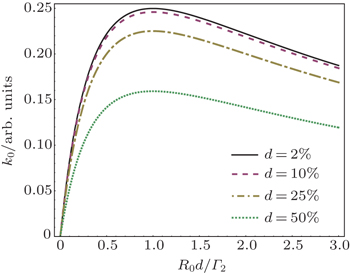
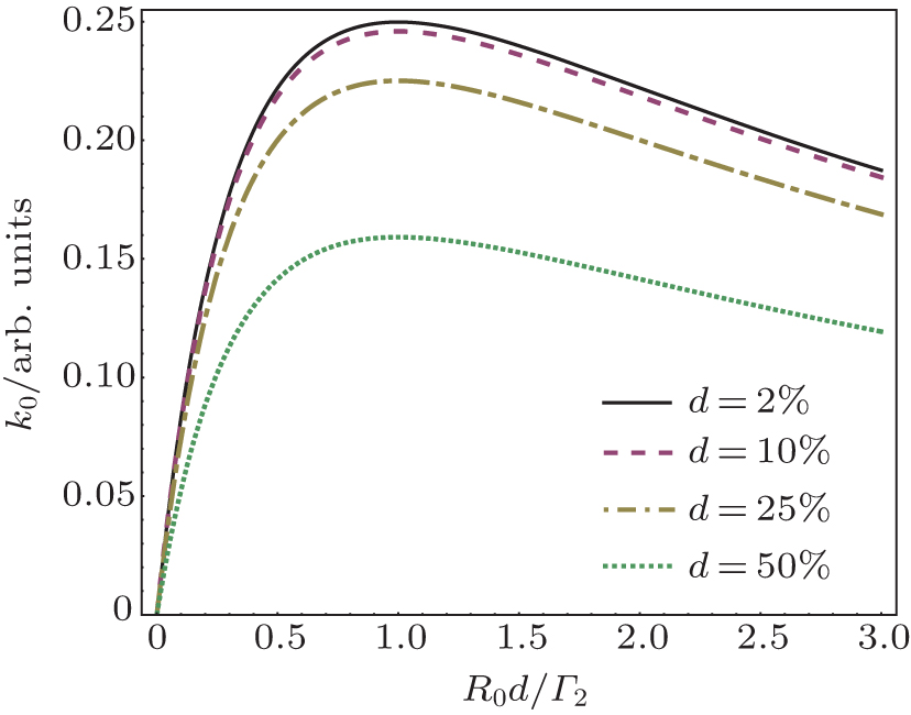
	Fig. 1. Dependences of the resonant response k0 on average pumping rate R0d for various duty cycles. The solid, dash, dash-dot, and dot lines are for d = 2%, 10%, 25%, and 50%, respectively.

For a fixed R₀, the maximum value of k₀ achievable by varying d, which we denote by , is obtained when cot (πd) = 2R₀/πΓ. The dependences of k₀ on d for various pumping rates are plotted in Fig. 2. It shows that increases with pumping rate and approaches to the ultimate limit , when R₀ ≫ Γ₂ and R₀d = Γ₂. We can see that for practical purpose, by choosing R₀ ∼ 10Γ₂ and d ∼ 10%, one can obtain a field response larger than 0.95.

Fig. 2.

	Figure Option ViewDownloadNew Window
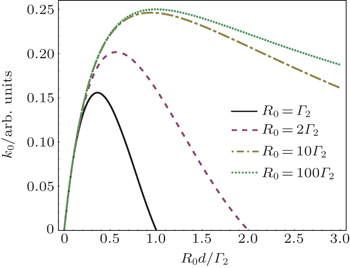
	Fig. 2. Dependences of the resonant response k0 on average pumping rate R0d for various pumping rates. The solid, dash, dash-dot and dot lines are for R0 = Γ2, 2Γ2, 10Γ2, and 100Γ2, respectively.

It is interesting to compare the result of square-wave AM with that of sinusoidal AM where R(t) = R₀+R₀ cos (ωt). One can find that for sinusoidal AM, the maximum field response is obtained at R₀ = Γ₂ and is equal to M₀/8Γ₂, which is only half of the for square-wave AM.

After having studied the effect of pumping on the field response, we turn to its effect on the noise. The noise δϕ is generally contributed by the photon shot noise of the probe beam, the spin projection noise of the atoms, light shift back-action noise and other technical noises.^[19] Here we only consider the possible noise related to the pumping parameters. Since β is independent of the pumping parameters, we have

To study the noise of μ due to fluctuation of pumping rate, we differentiate Eq. (9) with respect to R₀ using Eq. (4) and obtain

We will show that under our experimental conditions the above noise is already smaller than the spin projection noise δμ_sp.

Similarly, we can derive the noise of μ due to fluctuation of the duty cycle. Keep in mind that, in practice, δd is usually independent of d. Assuming Δ ≪ Γ, we have

One can see that δμ_d is also insensitive to the fluctuation of d at resonance. In the case of Δ ≠ 0, δμ_d is also proportional to 1/R₀ for large R₀. However, when R₀d = Γ₂ = Γ/2 and d ≪ 1, we have

We see that δμ_d can be tuned down by d until it becomes negligible compared with other noises.

We conclude that because the dispersive signal μ is insensitive to the fluctuation of pumping parameters near resonance, pumping induced noises are usually smaller than other fundamental noises in practice. Thus the optimal pumping condition for the sensitivity of AM BBM is R₀d = Γ₂ and d → 0, where the resonant field response |∂μ/∂Δ|_{Δ = 0} is maximized.

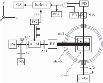
To verify our theory we conducted the following experiment. The schematic design of the experimental setup is shown in Fig. 3. A 24 mm × 24 mm × 24 mm cubic Pyrex cell containing isotopically enriched Rb (99.5 at.% ⁸⁷Rb) was placed in a ceramic oven at room temperature. The inner wall of the cell was coated with Octadecyltrichlorosilane (OTS).^[23] to reduce the wall relaxation. The cell was filled with 5 Torr (1 Torr = 1.33322×10² Pa) N₂ buffer gas to increase the optical pumping efficiency by velocity changing collisions and radiation quenching. The oven was mounted in a 4-layer cylindrical μ-metal shield. Three pairs of Helmholtz coils inside the shield provided a uniform magnetic field in the z direction. The inhomogeneity of the field was measured and negligible when the field strength was below 2 mGs (1 Gs = 10⁻⁴ T), which corresponds to a Larmor frequency of 1.4 kHz for the ⁸⁷Rb ground state. Our experiments were performed at a Larmor frequency of 1181 Hz. Two 795-nm distributed feedback (DFB) lasers resonant with the F = 1 → F′ = 2 and F = 2 → F′ = 2 transitions were combined into a single pump beam propagating along the x axis. The intensity of the pump beam was square-wave modulated by an acoustic optical modulator (AOM) controlled by a function generator. Neutral density filters are to be inserted behind the AOM to change the pump intensity, hence R₀. The pump beam was circularly polarized by a linear polarizer followed by a quarter-wave plate. Finally the beam was expanded to 2 cm in diameter to cover almost the entire cell. The intensities of the two DFB lasers were adjusted to be equal throughout the experiment to minimize the hyperfine polarization. An external cavity diode laser (ECDL) traversing the cell in the y direction served as a probe beam. The probe frequency was red-detuned about 2.5 GHz from F = 2 → F′ = 2 resonance. We used such a large detuning, which is about 10 times the optical Doppler half width, in order to avoid any complication caused by the absorption of the probe light. The beam diameter and the power of the probe was 2 mm and 6 μW respectively. The PFR of the probe transmission was detected using a balanced photo-detector behind a Walleston prism, whose homodyne output was fed separately into a spectrum analyzer and a lock-in amplifier referenced to the AOM modulation. The dispersive signal of PFR was obtained from the lock-in amplifier with a 3-ms time constant by scanning the modulation frequency over 400 Hz across the resonance in 4 s.

Fig. 3.

Figure Option ViewDownloadNew Window

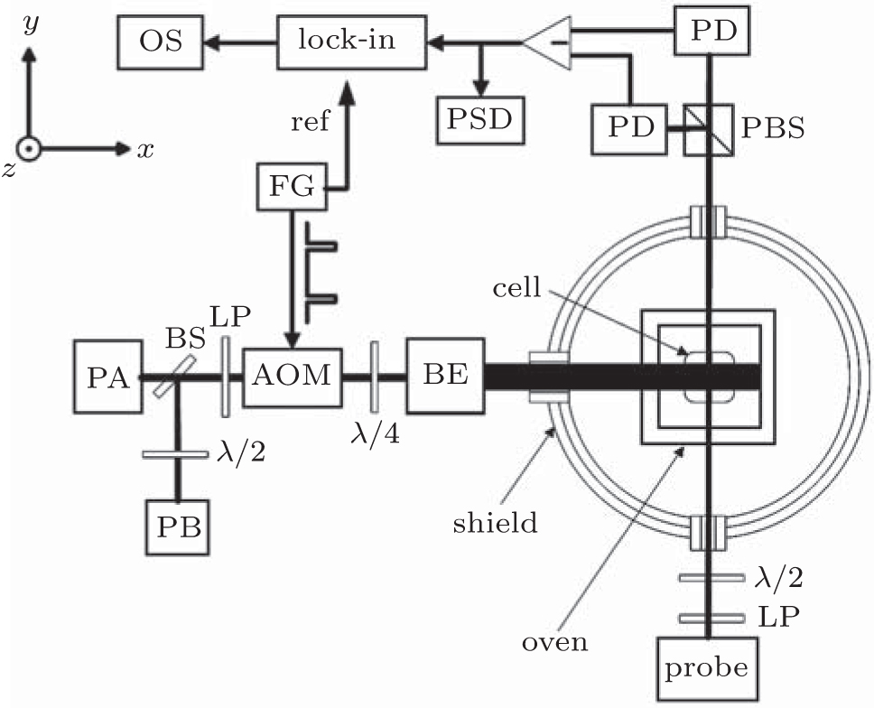
Fig. 3. Experimental setup. PA, PB: DFB lasers resonant with 87Rb D1 F = 2 → F′ = 2 and F = 1 → F′ = 2 transitions respectively, BS: beam splitter, LP: linear polarizer, AOM: acousto-optic modulator, λ/4: quarter-wave plate, λ/2: half wave plate, BE: beam expander, Shield: magnetic shield composed of four layers of mu-metal, Probe: probe laser, PBS: polarizing beam splitter, PD: photon detector, Lock-in: lock-in amplifier, FG: function generator, ref: AOM modulation trigger signal for lock-in reference, PSD: spectrum analyzer for power spectral density, OS: digital oscilloscope.

Figure 4 shows two typical PFR signals obtained in the experiment along with their fittings using Eq. (9). The pump power is 4.2 mW and duty cycles are 1.2% and 0.03%, respectively. One can see that the fitting to the data of the larger duty cycle is not so good as that of the smaller one. It is a general trend of our data that the line shape of the signal deviates from the pure Lorentzian profile of Eq. (9) when R₀d approaches to Γ₂, and becomes more distorted with increasing R₀d, the reason for which will be discussed later.

Fig. 4.

	Figure Option ViewDownloadNew Window
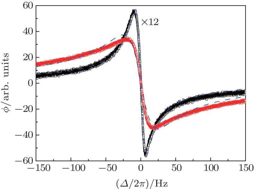
	Fig. 4. The experimental field response signals of Faraday rotation and their fittings using Eq. (9). The pump light intensity is 4.2 mW. The black squares and red circles represent the data for duty cycles of 0.03% and 1.2%, respectively, the former is amplified by a factor of 12 for easy viewing. Blue dash lines represent the fittings.

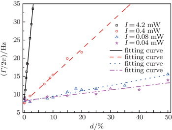
The dependences of the linewidth Γ on duty cycle for various pumping rates are measured and plotted in Fig. 5. The value of Γ is given by half the peak-to-peak frequency gap directly measured from the dispersive signal. The vertical intercept and the slope of the linear fit represent the fitted values of Γ₂ and R₀ respectively. Since our experiments were performed at room temperature where Γ_SE is less than 0.15 s⁻¹,^[24] the Γ₂ is mostly contributed by wall relaxation rate Γ_W.

Fig. 5.

	Figure Option ViewDownloadNew Window
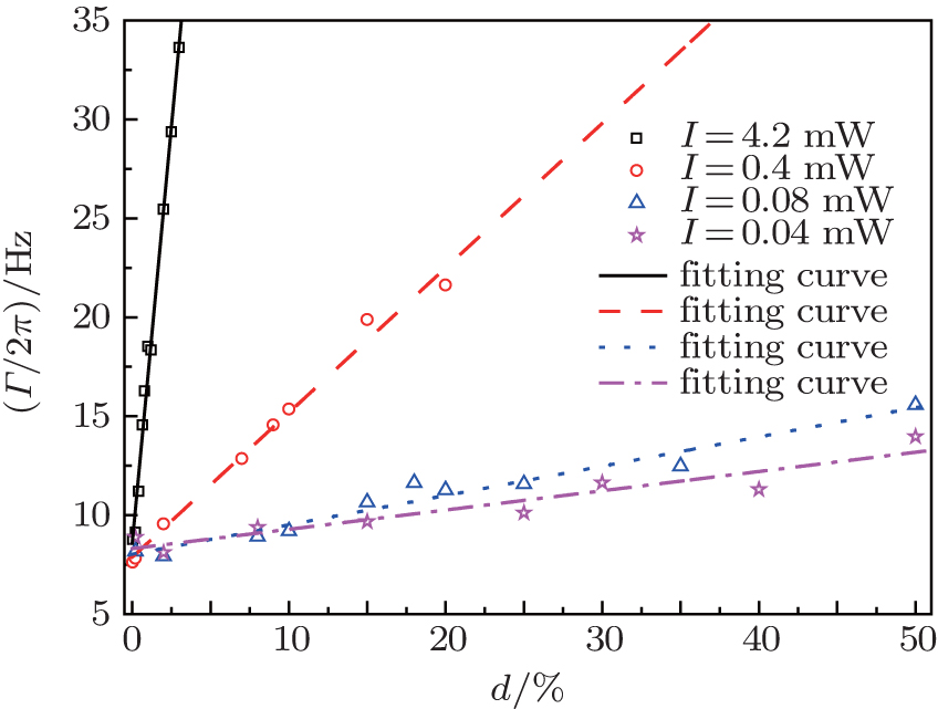
	Fig. 5. Experimental dependences of the linewidth on duty cycle for various pump powers. Blocks, circles, triangles and stars represent data taken under total pump powers of 4.2 mW, 0.4 mW, 0.08 mW, and 0.04 mW, respectively.

Figure 6 shows the dependences of the resonant response k₀ on duty cycle for the same set of data presented in Fig. 5. The resonant response is obtained from the slope of a linear fit of 100 data points near the resonance center of the PFR signal. At the same time the power spectral density (PSD) at resonance, measured by the spectrum analyzer, shows that the noise floor near resonant frequency is constant within several percents and independent of the duty cycle. Using the actual experimental condition: Γ₂ ≈ 10 2π · Hz, R₀ = 10Γ₂, d = 10%, Γ ≈ 20 2π · Hz, N_A = 10¹¹ and assuming some large fluctuations of the detuning, duty cycle and pumping rate: Δ = 1 2π · Hz, , , we can estimate that the pumping parameter related noises given by Eqs. (20) and (22) are smaller than the spin projection noise given by Eq. (19). By checking the probe intensity dependence of the same PSD, we find that the signal-to-noise ratio is proportional to the square root of the probe intensity, indicating that our system is actually limited by the photon shot noise of the probe.

Fig. 6.

	Figure Option ViewDownloadNew Window
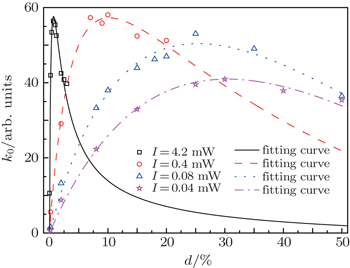
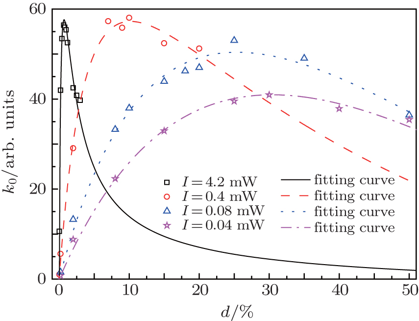
	Fig. 6. Dependences of the resonant response on duty cycle for various pump powers. Blocks, circles, triangles and stars represent experimental data taken under total pump powers of 4.2 mW, 0.4 mW, 0.08 mW, and 0.04 mW, respectively.

The fitted pumping rate and the optimal duty cycle obtained from the fittings are listed in Table 1. Notice that there is a discrepancy between the pumping rate obtained by fitting the duty cycle dependence of the linewidth and the resonant field response. Theoretically k₀ is related to Γ by Eq. (14). However when the average pumping rate exceeds the relaxation rate in the dark this relation will not hold exactly due to the hyperfine pumping effect. In our experiment, the probe beam is set to observe the MDM on the F = 2 hyperfine sublet mainly. However, inevitable hyperfine pumping will increase the population on the F = 2 sublet, causing M₀ to increase with increasing duty cycle, while in the current theory M₀ is assumed to be a constant. Such an effect causes the fitted pumping rate R_k to be bigger than R_Γ.

Table 1.

Table 1.

Table 1. Fitting parameters of the experimental data. IP is the total pump intensity. RΓ and Γ2 are respectively the R0 and the Γ2 obtained by fitting the data in Fig. 5. Rk and dk are respectively the R0 and the optimal duty cycle for obtained by fitting the data in Fig. 6. . IP/mW (Γ2/2π)/Hz RΓ/Γ2 dk/% Rk/Γ2 4.2 8.6 ± 0.4 98 ± 8 0.7 142 ± 6 0.4 7.9 ± 0.3 9.3 ± 0.7 10 9.1 ± 0.5 0.08 8.0 ± 0.3 1.8 ± 0.2 25 2.5 ± 0.2 0.04 8.3 ± 0.4 1.2 ± 0.2 30 1.7 ± 0.1

Table 1. Fitting parameters of the experimental data. IP is the total pump intensity. RΓ and Γ2 are respectively the R0 and the Γ2 obtained by fitting the data in Fig. 5. Rk and dk are respectively the R0 and the optimal duty cycle for obtained by fitting the data in Fig. 6. .

Large average pumping rate also causes a deviation of the experimental signal line shape from the pure dispersive Lorentzian profile given by Eq. (9) as can be seen clearly from the signal of the large pump intensity in Fig. 4. Since both the duty cycle and pumping rate are fixed in this case, this discrepancy cannot be explained by the reason as mentioned above. By tracing back the derivation of Eq. (9), we suspect that Eq. (5) is no longer accurate for describing the dynamics of MDM, because it might neglect some effect which is important at high average pumping rate. One possibility is the coupling between the evolutions of different spin polarization moments. For atoms with spin quantum number F, the circularly polarized pump light can generate spin polarization moments (PMs) of all ranks κ = 0,1,2, …, 2F.^[25] The precession frequency of a transverse PM of rank κ is equal to κ ω₀, so PMs of κ ≥ 1 are all synchronously pumped when the light modulation frequency matches the Larmor frequency ω₀. A weak probe can only detect PMs of κ = 0,1,2, which are named population, orientation and alignment respectively.^[25] The magnetic dipole moment probed by PFR at far optical detuning is only proportional to the orientation. For isotropic relaxations, PM of each rank evolves independently, but if the relaxation is anisotropic, PM’s of different ranks might couple to each other.^[26,27] Since the power broadening relaxation is anisotropic, it can cause couplings of PMs. For weak pumping, the magnitudes of higher rank PMs are negligible and the dynamics of orientation can be treated independently as described in Eq. (5). But when the average pumping rate exceeds Γ₂, the higher rank PMs become significant, and their coupling with the orientation might cause the deviation of its signal from a pure Lorentzian.

We theoretically study the dependences of the line shape of a square-wave amplitude-modulated Bell–Bloom magnetometer on the intensity and duty cycle of the pump light. We show that the maximum field response of the magnetometer can be achieved at the resonance center of the dispersive parametric-Faraday-rotation signal together on the condition that the duty cycle is small and the average pumping rate is approximately equal to the transverse relaxation rate in the dark Γ₂. The theoretical results are in agreement with experimental results for pumping rates ranging over two orders of magnitude above Γ₂. We also show that the signal at resonance is insensitive to the fluctuations of pumping rate and duty cycle. Thus it is the same condition for both the maximum field response and the optimal sensitivity. The line shape of experimental signal starts to deviate from the prediction of the theory when the average pumping rate exceeds Γ₂. A full density matrix calculation, which includes the hyperfine pumping and the dynamics of higher rank polarization moments is expected to give a more accurate description of this phenomenon.