
Cosine fitting radiography and computed tomography*
[Li Pan-Yuna), b) , Zhang Kaia)†  , Huang Wan-Xia
a) , Yuan Qing-Xia) , Wang Yana), b) , Ju Zai-Qianga), b) , Wu Zi-Yua) , Zhu Pei-Pinga), c)‡ ]
, Huang Wan-Xia]
|
|

 , Huang Wan-Xia
†Corresponding author. E-mail: zhangk@ihep.ac.cn
‡Corresponding author. E-mail: zhupp@ihep.ac.cn
*Project supported by the National Basic Research Program of China (Grant No. 2012CB825800), the National Natural Science Foundation of China (Grant Nos. 11205189, 11375225, and U1332109), the Knowledge Innovation Program of the Chinese Academy of Sciences (Grant Nos. KJCX2-YW-N42, Y4545320Y2, and 542014IHEPZZBS50659).
A new method in diffraction-enhanced imaging computed tomography (DEI-CT) that follows the idea developed by Chapman et al. [Chapman D, Thomlinson W, Johnston R E, Washburn D, Pisano E, Gmur N, Zhong Z, Menk R, Arfelli F and Sayers D 1997 Phys. Med. Biol.42 2015] in 1997 is proposed in this paper. Merged with a “reverse projections” algorithm, only two sets of projection datasets at two defined orientations of the analyzer crystal are needed to reconstruct the linear absorption coefficient, the decrement of the real part of the refractive index and the linear scattering coefficient of the sample. Not only does this method reduce the delivered dose to the sample without degrading the image quality, but, compared with the existing DEI-CT approaches, it simplifies data-acquisition procedures. Experimental results confirm the reliability of this new method for DEI-CT applications.
Since its introduction in 1973, [1] the absorption-based computed tomography (CT) has been widely used in many areas, such as medicine, industry, biology, and material sciences.[2– 5] However, this conventional CT method makes it impossible to resolve small features in soft biological tissues, which are mainly composed of low-Z elements and actually characterized by a small difference in the x-ray absorption cross section. On the contrary, x-rays penetrating into a material experience a considerably large phase shift. Thus, the use of the x-ray phase shift rather than the attenuation may allow achieving a substantially increased contrast. As a consequence, various phase contrast CT methods[6– 12] have been developed to sense the phase variations induced by a sample in the last two decades.
Diffraction-enhanced imaging computed tomography (DEI-CT), as one of the main phase contrast imaging technologies, is a recently developed imaging technique for radiography. It is easy to align, almost insensitive to mechanical drifts and provides a large field of view to image the whole specimen. Above all, DEI can be studied as a typical model among differential phase-contrast (DPC) imaging methods, [13– 16] and its research results can be generalized to other DPC imaging methods, especially to grating shear imaging which has hugely potential clinical applications, so studies on DEI have widespread and profound significance. However, studies performed with this technique need to collect several projective images for each projection view. The raw DEI projective images obtained in certain orientations of the analyzer crystal in the DEI system have much superposition information, including absorption, refraction, and ultra-small-angle x-ray scattering (USAXS). So collecting multiple DEI projective images to extract these three kinds of information from raw DEI images is needed before CT reconstruction.
Actually Chapman et al.[17] in 1997 developed the original DEI algorithm by linearly fitting the flanks of rocking curve (RC) to extract absorption attenuation and refraction-angle images from two DEI images in symmetrical positions of the Darwin width of the RC. Based on this method, the original DEI-CT method can present the two-dimensional (2D) and three-dimensional (3D) distributions of the absorption and refraction information.[8, 18– 21] However, the USAXS information of the sample, which is the refraction effects of an inhomogeneous area with smaller size than that of the resolution element, is neglected and cannot be reconstructed by the original DEI-CT method. The absence of USAXS information may possibly obscure important details of a low-Z sample, like soft tissue. In order to obtain the distribution of USAXS information of a sample, many recent studies offered some alternatives, either by collecting several images at different analyzer positions, [22– 27] called multiple-image radiography (MIR) which has high accuracy and strong ability to resist noise, or by providing a more general theory of ABI using wave-optical formalism.[28, 29] Apart from them, based on the original DEI algorithm, generalized diffraction-enhanced imaging (GDEI)[30] and improved diffraction-enhanced imaging (IDEI) method[31] can be combined respectively with a CT reconstruction algorithm to reconstruct absorption, refraction, and USAXS information in three different directions of the analyzer crystal.[32, 33] The two novel DEI-CT methods, each of which minimizes the dose delivered to the sample, have been confirmed by the strict theoretical derivation and many exciting experimental results in the past ten years.
Following Chapman’ s original idea, to simplify the expression of RC, herein, an alternative DEI-CT approach, based on the fit of RC with a cosine function limited by a window function to extract different information[34] and combined with the “ reverse projections” (RP) method, [35, 36] called the cosine-fitting radiography-based computed tomography (CFR-CT) method is proposed in this paper. Compared with the other DEI-CT methods, the CFR-CT method only needs to collect two sets of projective data in two defined directions of the analyzer crystal for each projection view, then the information about absorption attenuation, refraction angle, and USAXS of the sample can be extracted and the 3D distribution structure in the sample of the linear absorption coefficient, the decrement of the real part of the refractive index, and the linear scattering coefficient can be reconstructed. This approach not only simplifies image formulas and the image acquisition strategy, but also accelerates the computation time in data analysis without degrading the image quality.
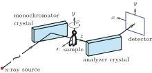
The setup of DEI-CT system as shown in Fig. 1, is composed of an x-ray source, a monochromator crystal, a rotational sample stage, an analyzer crystal, and a detector. The two coordinate systems are employed to describe the DEI-CT imaging system, the measurement coordinate system (x, y, z) is fixed on the detector, and the sample coordinate system (x′ , y′ , z′ ) is located on the sample (see Fig. 1). The relation between the two coordinates is as follows:
where φ is the rotation angle from x axis to x′ axis around the y axis, and the rotation axis of the sample and the analyzer crystal are both parallel to y axis.
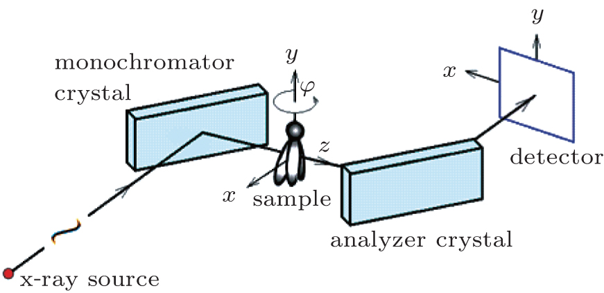 | Fig. 1. DEI-CT experimental set-up in BSRF. |
Based on the property of perfect-crystal reflection, only the angle in the meridional plane (x– z plane) can be detected, and that in the sagittal plane (y– z plane) is ignored. Consequently, all angles such as the incident angle, the reflection angle, and the rocking angle of the analyzer crystal in this study have been defined in the x– z plane.
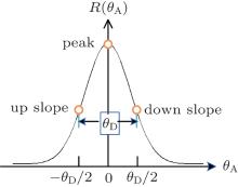
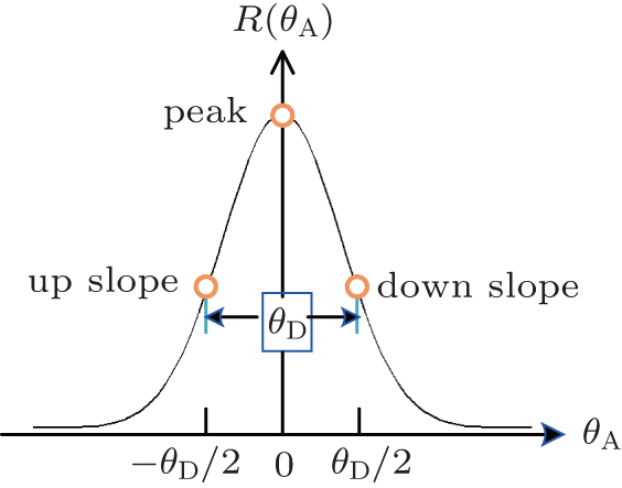 | Fig. 2. Rocking curve and its full width at half maximum (Darwin width) θ D. |
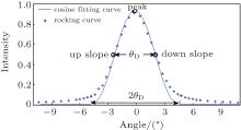
Converting the refraction angle and scattering angle induced by the sample into the change of detected intensity by the Rocking curve (RC) is the basic principle of the original DEI. The R(θ A) is the RC that describes the reflectivity versus the setting angle θ A of the analyzer crystal deflecting from the monochromatic crystal (see Fig. 2). Because the incident angle change of the ray on the analyzer crystal, caused by the refraction and scattering of the sample, is equivalent to that caused by rotating the analyzer crystal with respect to the ray, the RC describes the inherent ability of the DEI system to convert the angle signal induced by the sample into intensity. From Fig. 2, it is clearly observed that RC function curve segment is mainly within θ A ∈ (− θ D, θ D) and has almost no response outside the area. Because the original math expression of RC, deduced from the dynamics theory of crystal diffraction, is too complex[27, 37] to extract angle information directly, good fitting of RC with simple function is the important and efficient choice. Because of simple expression, periodicity, and symmetry in cosine function, our research group proposes using a cosine curve limited by a window function to fit the RC. The cosine curve limited by the window function can fit the RC very well (see Fig. 3), and this method may offer some advantages in obtaining an analytic formula to analyze intuitively the principles of physics, and in simplifying the extracting-information algorithm to accelerate the data-processing time. So, R(θ A) can be expressed as
where R̅ is the mean value of the RC, V0 = (Rmax − Rmin)/(Rmax + Rmin) is the visibility of the RC, Rmax and Rmin are the maximum and minimum value of RC, respectively.
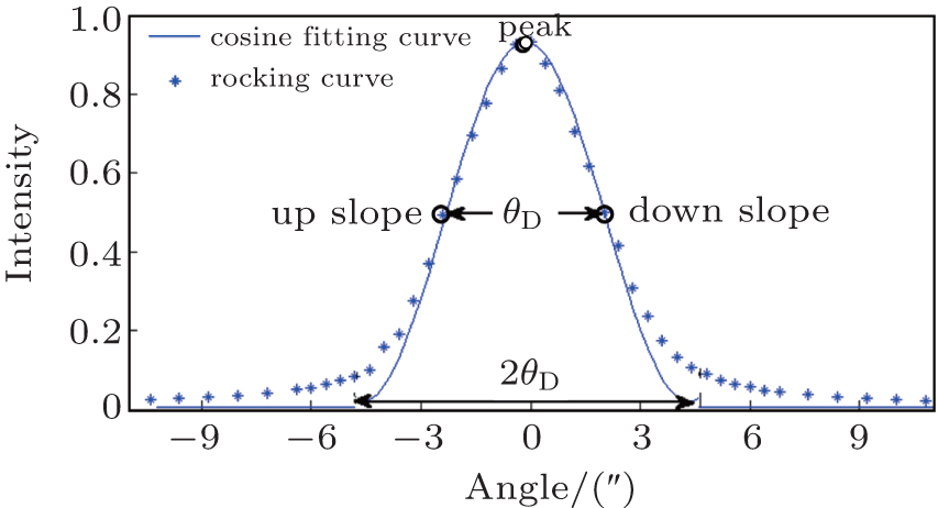 | Fig. 3. Comparison between the RC acquired in BSRF at 15 keV and its corresponding cosine-fitting curve. |
Based on Eq. (2), by rocking the analyzer crystal around the y axis without a sample in Fig. 1, the intensity I recorded by the detector can be expressed as
where I0 is the intensity of the x-ray beam incident on the sample plane.
When a sample composed of low-Z elements is placed in the DEI-CT system between the monochromator crystal and the analyzer crystal, the sample will absorb, refract, and scatter the x-ray beam illuminated.The angular intensity function f(θ A; x, y) of the transmitted beam induced by the sample can be expressed as[38]

where M(x, y) is the absorption of the sample point (x, y) with the expression

μ (x, y, z) is the linear absorption coefficient, θ (x, y) is the vertical component of the refraction angle, and is expressed as

where δ (x, y, z) is the decrement of the real part of the refractive index, σ 2(x, y) is the scattering variance of sample point (x, y) and expressed as[39]


where Δ zi is the thickness of the thin layer of the sample in the integral path, 

where ⊗ is the convolution. Because the refraction and scattering angle of a sample are mainly distributed in the range of less than θ D, and the sensitivity of the DEI system only depends on the detection of a small angle, regardless of a large angle signal, the width of the window function is limited to (− 0.5θ D, 0.5θ D) in the following discussion. Based on the above hypothesis and Eqs. (2) and (4), the detected intensity equation of DEI can be expressed as (see Appendix A for the specific derivation process)
where V(x, y) is the visibility of RC modulated by sample and its expression is
According to the above expression, V(x, y) is a measure of the effective integrated local small- (and ultrasmall-) angle scattering power of a sample. For homogeneous specimens, i.e., for a sample with negligible USAXS contribution, the value for the visibility equals V0 . However, for a specimen which exhibits a non-ignorable USAXS signal, it shows a significant decrease in the visibility and yields the value of V(x, y) < V0 . Apart from the conventional absorption information, the deflection angle between the analyzer crystal and the monochromator crystal, the refraction angle and scattering angle induced by the sample are reflected in the detected image intensity expression in Eq. (9) and thus offer additional contrast. That is, the imaging intensity function Iθ A, dubbed the “ angular signal response function” , expresses the response of the DEI system to different properties of a sample placed in system, especially to the deflection angle of transmitted beam induced by the sample. Various angular signal response curves in the DEI system can be obtained if θ A is given. Based on Eq. (9), the peak angular signal curve IP and downslope angular signal curve ID at projective view φ can be respectively established when analyzer crystal is fixed at θ A = 0 and θ A = θ D/2, respectively:
And the reverse angular signal curve of the downslope is


Combining Eqs. (11)– (13), the three properties of the sample can be expressed as

We now apply a filtered back-projection (FBP) algorithm.[40– 43] to the calculated parametric tomographic datasets M(x, y, φ ), θ (x, y, φ ), and σ 2(x, y, φ ) by using the cosine-fitting radiography (CFR) algorithm, three-dimensional (3D) parametric features of the sample can be obtained. Reconstruction formulas of μ (x′ , y′ , z′ ), δ (x′ , y′ , z′ ), ∂ δ (x′ , y′ , z′ )/∂ x′ , ∂ δ (x′ , y′ , z′ )/∂ z′ , and ω (x′ , y′ , z′ ) are respectively expressed as[43, 44]
where F and F− 1 denote Fourier transformation and its inversion, respectively, and δ ̃ is the Dirac function.
Of note is that the three properties of a sample can also be acquired by setting the orientations of the analyzer crystal at θ A = − θ D/2 and θ A = 0 to obtain the image equations of the peak IP (x, y, φ ), upslope IU (x, y, φ ) and IU (− x, y, φ + π ). That is to say, the CFR-CT method offers a simply way to reconstruct 3D information about absorption, refraction, and scattering from two sets of projection data: either the upslope or downslope image with the sample rotational angle from 0° to 360° , and the peak image with the rotational range from 0° to 180° .
The CFR-CT experiment was performed on the beamline 4W1A at Beijing Synchrotron Radiation Facility (BSRF). The DEI-CT set-up was constructed with two Si (111) crystals: the monochromator crystal served as an angular collimator with an acceptance angle of a few arcseconds: the full width of the Rocking curve, while the analyzer crystal was a narrow angular band-pass filter with the same high angular sensitivity. An x-ray energy of 15 keV was selected with the monochromator crystal and a charged coupled device camera with a pixel size of 7.4 µ m was used in this experiment. The biological sample was a front toe of a hamster which was approximately 4 mm in length, 2 mm in width, and 2 mm in thickness. A wealth of bone structure, muscle, and fur were contained in the sample. Raw images were acquired with an exposure time of 80 ms, a scan interval of 0.5° at two defined different positions, and outlined in Fig. 3 are the downslope image data with the sample rotational angle from 0° to 360° and the peak image data with the rotational range from 0° to 180° .
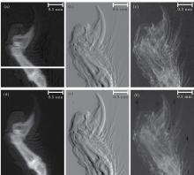
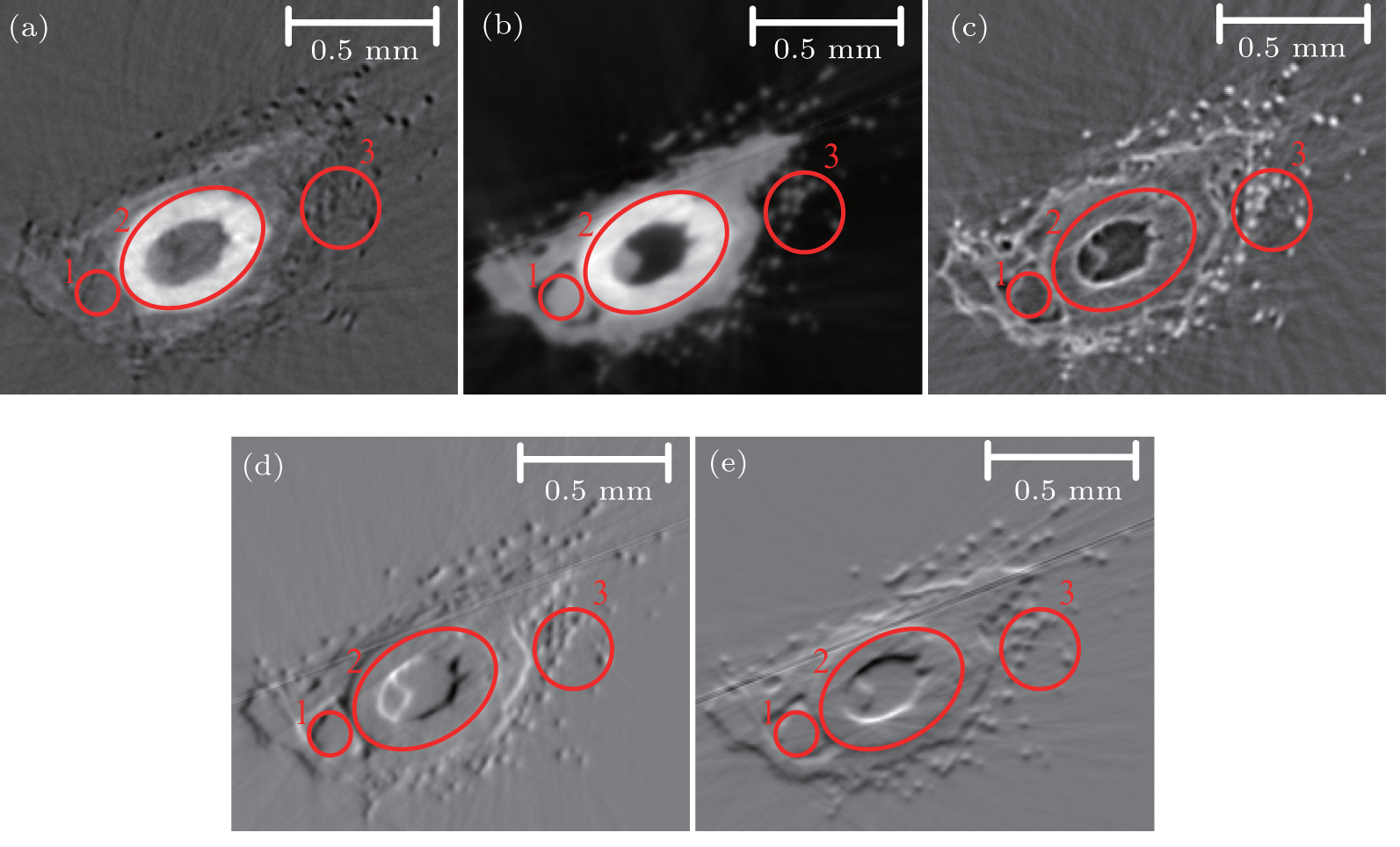
In order to demonstrate the feasibility of the CFR algorithm by comparing with MIR, 44 images were acquired with the analyzer crystal rotating from − 9.8 to 10 s along the RC at φ = 0. However, the basic parameters that the MIR algorithm used, i.e., the intensity of incident light, and the intensities after the light had been absorbed, refracted, and scattered by the sample point, were detected in only one detector pixel at different orientations of the analyzer crystal. Based on these parameters and the DEI setup in BSRF with a distance of 13 cm from the analyzer crystal to the detector and a pixel size of 7.4 µ m of the detector, the maximum angle deflection of the analyzer crystal was obtained to be about 5.9 s. So, multiple images were chosen to extract information by using the MIR algorithm with the analyzer crystal rotating from − 5.9 s to 5.9 s in this study. Figures 4(a)– 4(c) show the extracted M(x, y, 0), θ (x, y, 0), and σ 2(x, y, 0) of sample by using the CFR algorithm, while what figures 4(d)– 4(f) show are obtained by using the MIR algorithm. The quantitative comparisons of these methods are shown in Fig. 5.
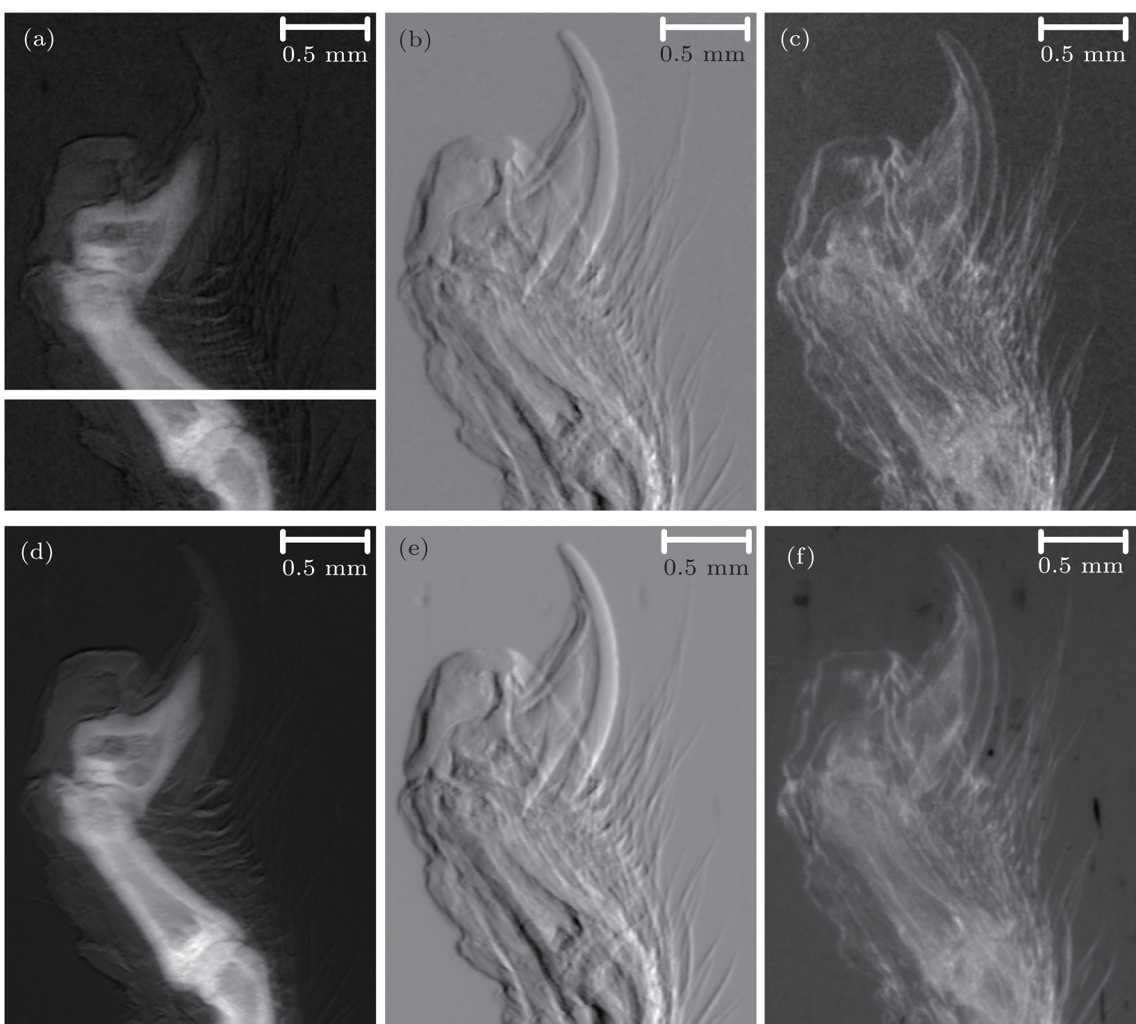 | Fig. 4. Images extracted by CFR and MIR algorithms. Panels (a)– (c) contain images obtained by using the CFR algorithm that depict M(x, y, 0), θ (x, y, 0), and σ 2(x, y, 0), respectively. The corresponding images obtained by using the MIR algorithm are shown in panels (d)– (f), respectively. |
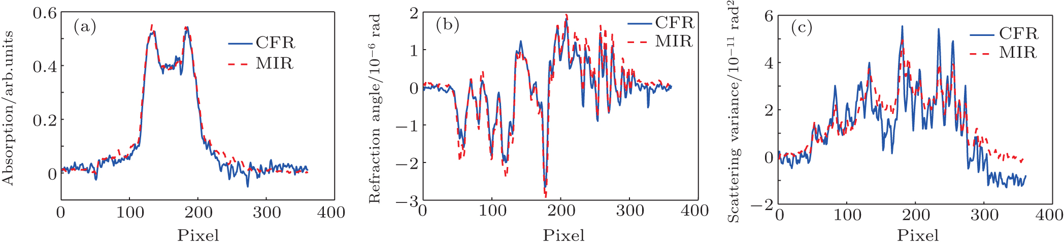 | Fig. 5. Profiles (corresponding to the horizontal white line across sample in Fig. 4) showing the comparisons of (a) absorption, (b) refraction angle, and (c) scattering variance between CFR and MIR methods. |
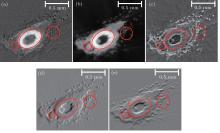
In Fig. 5, the quantitative information of absorption, refraction angle, and scattering variance shows those quantities obtained by CFR and MIR methods are quite consistent with each other, which verifies the feasibility of the CFR method. Based on the reconstruction equations (17)– (21), figure 6 shows the reconstructed slice images of μ (x′ , y′ , z′ ), δ (x′ , y′ , z′ ), ω (x′ , y′ , z′ ), ∂ δ (x′ , y′ , z′ )/∂ x′ , and ∂ δ (x′ , y′ , z′ )/∂ z′ corresponding to the horizontal white line across the sample in Fig. 4, respectively.
As shown in Fig. 6, valuable information can be obtained by using the CFR-CT method. Comparing the zooms in region 1 and region 2 of the absorption, the refraction, and the scattering information of the sample in Fig. 6, refraction and scattering information show a greatly improved contrast in soft tissue. The bone structure marked with white spots in Fig. 6(a) is well depicted in the absorption information, since bone has a higher linear absorption coefficient than other structures. In Figs. 6(b), 6(d), and 6(e), imaging contrasts in the slice of the refractive index and its derivatives are all highly enhanced: the soft tissue surrounding the bone structure as well as fur shown in dots, is easier to discern from the background than the absorption one. The components with a high linear scattering coefficient, like fur, and the edges of the different objects give a strong scattering signal. The fur signed as white spots in Fig. 6(c) is clearly visible.
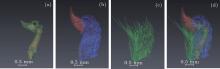
In order to obtain a more intuitive description and detailed information, the sample was divided into four parts: bone structure, tiptoe, muscle, and fur. As shown in Fig. 7, each part was extracted from its relatively abundant expression among the different information by the software of Avizo.
 | Fig. 6. Axial slices of the biological sample extracted with the CFR-CT method: (a) μ (x′ , y′ , z′ ), (b) δ (x′ , y′ , z′ ), (c) ω (x′ , y′ , z′ ), (d) ∂ δ (x′ , y′ , z′ )/∂ x′ , and (e) ∂ δ (x′ , y′ , z′ )/∂ z′ . Zooms shown in regions 1, 2, and 3 show respectively the tendons, bone structure, and the fluff of the sample. |
 | Fig. 7. 3D features of the four extracted segments of a sample from different information: (a) bone structure from absorption information, (b) tiptoe and muscle from refraction information, (c) fur from scattering information, and (d) combined four segments of the sample from different information. |
In fact, the original DEI method developed by Chapman et al. is based on fitting the RC with a trigonometric function, so that the absorption and refraction properties of a sample can be extracted via an analytical solution. Following this idea, to simplify the expression of RC, the CFR-CT method, an alternative choice to extract absorption, refraction, and scattering properties of a sample based on DEI technology has been investigated by our group. At the same time, we demonstrated that the CFR-CT method yields comparable absorption, refraction, and scattering information to those the MIR-CT method produced at the same projection view.
However, the basic hypothesis concerning the imaging principle of extracting different information of a sample in DEI needs to be stressed: all the photons exiting from the object plane at one point of the sample are absorbed, refracted, and scattered by the sample point and will be collected by a certain pixel of the detector. That is to say, the refraction, and the scattering angle caused by the sample point need to be smaller than the opening angle of a resolution cell of the detector to the sample point. Thus, the deflection angle range of analyzer crystal should be calculated and chosen before using the CFR method and MIR method.
Another issue is about locating accurately the positions of the upslope and the peak or the downslope and the peak when using the CFR-CT method, especially at the narrower FWHM of the RC with the rise of energy in DEI. Accompanied with mechanical error and the drift of light, all these factors make it more difficult to accurately locate the positions we need at high energy in the DEI setup. To overcome the problem, maybe a higher precision crystal turntable is needed. We are presently assessing how large a deflection angle error of the analyzer crystal, when locating these positions, is acceptable with some degree of statistical accuracy to extract the absorption, refraction, and scattering parameters in the CFR-CT method. Furthermore, a more sensitive angle response will be introduced with the narrower FWHM of the RC, which may be studied in the DEI imaging field with higher spatial resolution.
In general, all existing methods to extract different information of a sample in a DEI experiment can be summarized as two philosophies. One is fitting the RC with a certain function pioneered by Chapman et al.[17] The essence of this philosophy is to deduce the imaging equation analytically by convolving the angular intensity function of the transmitted beam induced by the sample and the fitting-RC function. The other philosophy represented by Wernick et al.[22, 25] is developed by acquiring several images at different analyzer positions. By comparing quantitatively the RCs measured with and without the sample pixel by pixel, the different information of the sample can be obtained.
Following the former philosophy, a novel approach called the CFR-CT method is proposed, which adopts the cosine function limited by a window function to fit the RC and combines the RP algorithm to reconstruct the 3D distribution of the linear absorption coefficient, the decrement of the real part of the refractive index, and the linear scattering coefficient. Compared with the original DEI-CT method, the CFR method takes the scattering information into account, while the original DEI-CT does not. Furthermore, the CFR-CT method obtains almost a similar result to the MIR-CT method, which is proven by qualitatively and quantitatively comparing the experimental results. Compared with the GDEI-CT and IDEI-CT methods, the CFR-CT method only needs two projection datasets at two defined directions of the analyzer crystal to reconstruct the absorption, refraction, and scattering information, which simplifies image formulas and the image acquisition strategy, but also accelerates the computation time in data analysis without degrading the image quality. Therefore, the CFR-CT method can be considered as an alternative method of observing 3D information of a sample not only in DEI-CT, but also in other differential phase contrast imaging-based CT, such as grating shearing imaging and so on, which is particularly attractive in clinical radiography and in medical imaging.
| 1 |
|
| 2 |
|
| 3 |
|
| 4 |
|
| 5 |
|
| 6 |
|
| 7 |
|
| 8 |
|
| 9 |
|
| 10 |
|
| 11 |
|
| 12 |
|
| 13 |
|
| 14 |
|
| 15 |
|
| 16 |
|
| 17 |
|
| 18 |
|
| 19 |
|
| 20 |
|
| 21 |
|
| 22 |
|
| 23 |
|
| 24 |
|
| 25 |
|
| 26 |
|
| 27 |
|
| 28 |
|
| 29 |
|
| 30 |
|
| 31 |
|
| 32 |
|
| 33 |
|
| 34 |
|
| 35 |
|
| 36 |
|
| 37 |
|
| 38 |
|
| 39 |
|
| 40 |
|
| 41 |
|
| 42 |
|
| 43 |
|
| 44 |
|