A theoretical exploration of the influencing factors for surface potential*
[Liu Xin-Mina), b) , Yang Ganga)†  , Li Hang
a)‡ , Tian Ruia) , Li Ruia) , Ding Wu-Quana) , Yuan Ruob) ]
, Li Hang, Tian Rui|
|


†Corresponding author. E-mail: theobiochem@gmail.com
‡Corresponding author. E-mail: lihangswu@163.com
*Project supported by the National Natural Science Foundation of China (Grant Nos. 41371249, 41201223, and 41101223) and the Fundamental Research Funds for the Central Universities, China (Grant No. XDJK2015C059).
Although it has been widely used to probe the interfacial property, dynamics, and reactivity, the surface potential remains intractable for directly being measured, especially for charged particles in aqueous solutions. This paper presents that the surface potential is strongly dependent on the Hofmeister effect, and the theory including ion polarization and ionic correlation shows significant improvement compared with the classical theory. Ion polarization causes a strong Hofmeister effect and further dramatic decrease to surface potential, especially at low concentration; in contrast, ionic correlation that is closely associated with potential decay distance overestimates surface potential and plays an increasing role at higher ionic concentrations. Contributions of ion polarization and ionic correlation are respectively assessed, and a critical point is detected where their contributions can be exactly counteracted. Ionic correlation can be almost neglected at low ionic concentrations, while ion polarization, albeit less important at high concentrations, should be considered across the entire concentration range. The results thus obtained are applicable to other interfacial processes.
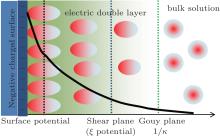
Surface potential is at the Stern plane of charged particles (Fig. 1) and has been used to probe the interfacial properties, dynamics, and reactivity. A number of methods based on zeta (ξ ) potential, [1, 2] negative adsorption, [3] positive adsorption, [4, 5] and pH indicator[6] have been used to obtain surface potential. It has important implications for a variety of nano/colloidal systems such as clay minerals, proteins, and membranes. Notwithstanding, for these charged particles in aqueous solutions, the direct measurement of surface potential remains a difficult task, and hence zeta (ξ ) potential that obviously has a small value is often used to represent surface potential[7– 9] (see Fig. 1). On the other hand, not a few theories have been developed to predict surface potential, such as Poisson– Boltzmann theory, [4, 5, 10] self-consistent field theory, [11] classical density functional theory, [12– 14] and integral-equation theory.[15]
Generally, the theories currently used to predict surface potential overlook Hofmeister (or specific ion) effects. Specific ion effects, which were first observed about 120 years ago, have been found to be ubiquitous and play a central role in physical, chemical, biological, and colloidal sciences.[16– 18] A variety of experimental phenomena can be explained by use of ion specificities, such as DNA conformation and stability, [16, 19– 21] activity coefficient, [22] interfacial tension of electrolyte solutions, [23, 24] colloidal forces, [25, 26] and buffer.[27, 28] Through the effects of interactions between ions and charged surfaces, ions and ions as well as ions and solvent molecules, the specific ion effect exhibits pronounced influences on the distributions of ions at the interface and in bulk solutions, [29] which further alters the results of surface potential. Therefore, it is no wonder that classical theories that neglect Hofmeister effects are unlikely to make a sound prediction.[28– 30] The surface potential expression with the inclusion of specific ion effects due to the enhanced ion polarization in the diffuse layer has recently been derived in our laboratory; [31, 32] however, the physical meanings of the ion polarization and ionic correlation in this expression remain ambiguous, and such investigations are of necessity in order to promote our understanding of surface potential; meanwhile, insightful clues can be provided towards its direct measurement.
In the present work, the respective contributions of ion polarization and ionic correlation to surface potential are also evaluated for the various colloidal systems and a wide range of ionic concentrations. Strong ionic correlation between condensed counterions can lead to attractive interaction among colloidal particles[33] as well as charge reversal.[34] On the other hand, ionic correlation at high salt concentrations can reduce the counterion concentration in the diffuse layer.[35] This adds the difficulty in measuring the surface potential because ionic correlation usually works in a collaborative manner with ion polarization. We are not aware which is more important for the surface potential determination, ion polarization or ionic correlation. How these two factors behave at different ionic concentrations also remains unclear to us. In the meantime, surface potential decays gradually in the electric double layer (Fig. 1), and the relationship between the potential distribution and decay distance is explored, which helps to understand the difference from zeta (ξ ) potential. To address the above issues, the rest of this paper is organized as follows. In Section 2, we show the theoretical surface potential expressions with only Coulomb force as well as correction by ionic correlation, ion polarization, and both factors. In Section 3, the presence of strong ion polarization is evidenced, and then the respective contributions of ionic polarization and ionic correlations are evaluated. In Section 4 the main conclusions are drawn from the present study.
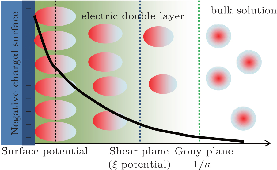 | Fig. 1. Counterion distribution, relative positions of surface, and zeta (ξ ) potentials as well as schematic representation of these potentials, each as a function of the potential decay distance that starts from the charged surface and extends towards the bulk solutions (thick solid curve). |
In this section, the various surface potential theories that are developed on the basis of the Poisson– Boltzmann (PB) equation are elaborated. For a given system, ion polarization and ionic correlation usually function collaboratively, and are intractable to distinguish for the experimental researchers.
For a binary electrolyte system, ions in the diffuse layer should abide by the Boltzmann distribution,

where 
The mean ion concentration in the diffuse layer equals

where Ni (mol· g− 1) is the amount of the i ion that interacts with the charged particle surface, S (dm2· g− 1) is the surface area of the charged particle, and κ (dm− 1) is the Debye– Hü ckel parameter.
In our previous work, [36] the potential distribution φ (x) of the binary electrolyte system containing monovalent and divalent counterions (e.g., NaCl + CaCl2) was derived on the basis of the nonlinear Poisson– Boltzmann (PB) equation,
where
In Eq. (4), φ 0 represents the potential at the original plane of the diffuse layer (or Stern plane), and here is regarded as surface potential (see Fig. 1).
Introducing the potential distribution function into Eq. (1) and then combining Eq. (2), we arrived at

with

In Eq. (5), ε is the dielectric constant of water (8.9× 10− 10 C2· J− 1· dm− 1), F (C· mol− 1) is the Faraday constant, m, also referred to as 


Then the following expressions can be derived for the binary system (i and j)

As a result, the surface potential of the classical theory 

Equation (8) is the derivative of the original PB equation where only Coulomb interaction occurs between ions and surface.
It is apparent that ionic correlation affects the ion-exchange process and hence this factor should be taken into account:[38, 39]

where μ i0 is the standard chemical potential, while 


The chemical potential in the diffuse layer can be written as

where 

According to the previous studies, [31, 37, 41] ionic activity represents a function of the Coulomb energy 
When the ion exchange process reaches equilibrium, we have 

In consideration of ionic correlation, the PB expression is modified into
Expressions similar to Eq. (7) can be derived as

where

As a result, surface potential with the inclusion of ionic correlation is

It can be seen from the above descriptions that the ionic activity in solution has been taken into account by considering ion size and ionic dispersion potentials of ion– ion and ion– interface interactions.[28]
As is well known, strong electric fields (108 V· m− 1 ∼ 109 V· m− 1) often exist at the surfaces of colloidal particles.[31, 32, 42– 50] As reported previously, the strongly polarizable ions can be adsorbed on the air– water and oil– water interfaces thus affecting the interfacial tensions.[23] For the negatively charged colloidal particles, the ions at their interfaces should be polarized more significantly, [51, 52] and the addition of polarization energy 

The above equation can be further transformed into[53]

with
where 
The exponential term in Eq. (18) equals
Then the coefficients β i and β j are

The coefficients β i and β j represent functions of the dipole moment difference 

At low ionic concentrations, the effect of ionic activity can be neglected, that is, 


The specific ion effects due to ion polarization are embodied with coefficients β i and β j, which are sensitive to the choice of ion pairs because ion polarizabilities in the diffuse layer are probably different.[29] Note that
The coefficients β Na and β Ca can be derived from Na+ – Ca2+ exchange equilibrium experiment, [43] and their empirical expressions are 


On the other hand, according to the classical theory, the polarization effect for a given ion and the polarization difference between Ca2+ and Na+ are estimated by


where

ε 0 is the dielectric constant in a vacuum and ε i = 1 + 4π α i/Vi, [55]
Figure 2 shows the polarization differences between Ca2+ and Na+ ions, obtained by the experimental electric double layer 


 | Fig. 2. Polarization differences between the Ca2+ and Na+ ions (  |
It is worth noting that the water should be also polarized by a strong electric field, [57] but which is obviously less than the charge dipole such as Ca2+ and Na+ ions; [58– 60] that is, the water solvent has a limited influence on the interactions between ions and surface charges that are mainly responsible for specific ion effects. Moreover, the influence of the ionic solution has already been included in the surface potential expression by ionic correlation (for the details, see Subsection 2.2.).
Si4+ and Al3+ are the principal constituents for most clay minerals, and isomorphous substitutions with metal ions of almost the same radii create permanent negative charges, e.g., usually the substitutions of Mg2+ /Al3+ for montmorillonite. It seems very difficult for lattice cations to be replaced by ions from the surfaces and bulk solutions, especially Ca2+ and Na+ that have substantially larger radii than Si4+ and Al3+ . Table 1 lists the surface potentials of montmorillonite (mean size: 1480 nm) and rutile titania (TiO2, mean size: 25 nm), [32] that have been calculated by the various schemes in Section 2, i.e., the classical theory (


Polarization and gathering of counterions in proximity to the negatively charged surfaces cause an enhancement of the shielding effect on the surface charges, which further leads to a substantial decrease to surface potential. It is in good agreement with the predicted result of ion polarization. Instead, few researchers[55, 56, 61– 63] insist that Hofmeister effects should result from the dispersion energy and ionic steric effect that are known to be significant only in the case of relatively high ion concentration. This seems to be a discrepancy with the fact that Hofmeister effects are more evident at low ionic concentrations due to the more pronounced enhancement of ion polarization in the electric double layer. With inclusion of ion polarization, the surface potentials (
| Table 1. Values of ionic strength (I) of solution containing Na+ and Ca2+ ions and surface potentials (φ 0) for montmorillonite and rutile titania (TiO2) suspended in these solutions that are obtained by the various schemes in Section 2. Units of ionic strength and surface potential are mmol· L− 1 and mV, respectively. |
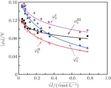
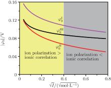
Figure 3 shows the variations of surface potentials for illite, i.e.,


The correlation coefficients (R2) given in Eqs. (27)– (30) indicate that these fitted functions describe reasonably the relationships between surface potentials (
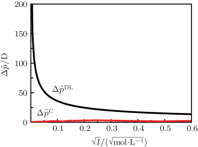
The contribution of ion polarization 
Therefore, ion polarization in the electric double layer strongly affects the surface potential and its contribution is quantitatively evaluated. The surface potential decays gradually within ionic solution, and then the potential distribution φ (x) can be described by the nonlinear PB equation.[36]
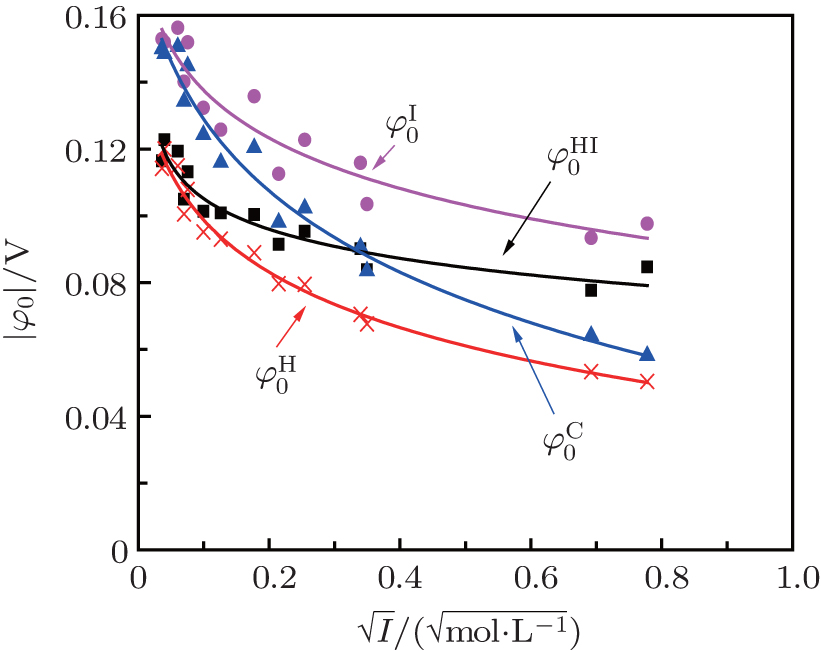 | Fig. 3. Variations of surface potentials (φ 0, in unit V) of illite in ionic solutions with root square of ionic strength ( |
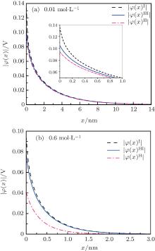
The surface potential decays gradually within ionic solution, and the potential distribution φ (x) does not need to additionally consider the ion polarization because this factor has already been accounted for during the calculation of surface potential. In order to investigate the relationship between potential distribution and ionic concentration, two ionic strengths (0.01 mol· L− 1 and 0.6 mol· L− 1) are selected for the NaCl + CaCl2 mixed solution 
The φ (x)H and φ (x)HI potentials approach to the null point at x = 2.40 nm for I = 0.6 mol· L− 1 whereas at x = 13.3 nm for I = 0.01 mol· L− 1, indicating an apparently faster decay rate at higher ion concentrations. In addition, at a given ionic strength, the φ (x)H and φ (x)HI potentials that include ion polarization vanish at the identical distances as the φ (x)I potential. This demonstrates that the forces generated by the surface charges are independent of ion polarization. At low concentrations (e.g., I = 0.01 mol· L− 1 in Fig. 4(a)), ion polarization makes an important contribution to the surface potential and potential distribution, and the inclusion of only ion polarization in the electric double layer is already sufficient to obtain reasonable results as indicated by the comparable φ (x)H and φ (x)HI data (Fig. 4), which accord with the surface potential data shown in Table 1 and Fig. 3. However, at relatively high concentrations (e.g., I = 0.6 mol· L− 1 in Fig. 4(b)), the φ (x)H results seem to deviate significantly from those of φ (x)HI, and it suggests that only the ion polarization effect cannot correctly account for the surface potential nor potential distribution, which will be discussed in the following.
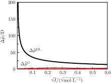
As indicated in Fig. 3, surface potentials including ionic correlation in bulk solution 

It can be found that at high ion concentrations, ionic correlation affects surface potentials even more apparently than ion polarization (Fig. 3). For example, at I = 0.6 mol· L− 1, 

Figure 4 shows that the potential distribution with considering the ionic correlation [φ (x)I] becomes obviously less with the increase of decay distance (x), and the decay rates of φ (x)I are more dramatic at higher ion concentrations. As discussed in Subsection 3.2, at a given ionic strength, the φ (x)I, φ (x)H, and φ (x)HI potentials vanish at the same distances that are strongly concentration-dependent, that is, these potentials are equal to zero at x = 2.40 nm for I = 0.6 mol· L− 1 while x = 13.3 nm for I = 0.01 mol· L− 1, respectively. This is assertive evidence for the association of concentration-associated ionic correlation for surface potential with the potential distribution. Accordingly, ionic correlation in bulk solution should be included when determining the surface potential and potential distribution.
At rather low ionic strengths (I ≤ 0.01 mol· L− 1), the polarization effect predominates during the determination of surface potential and potential distribution, whereas the effect of ionic correlation can be almost neglected (Figs. 3 and 4). With the increase of ionic strength, each of these two effects plays a definite role and it is their synergy that results in the accurate surface potential and potential distribution. Compared with the referenced  ;
; 

 | Fig. 4. Variations of the potential distribution (∣ φ (x)∣ , in V) with decay distance (x, in nm) at two different values of ionic strength (I): (a) 0.01 mol· L− 1 and (b) 0.6 mol· L− 1. |
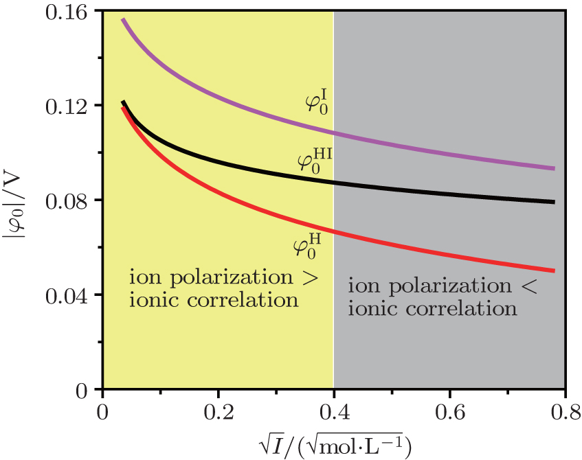 | Fig. 5. Illustration of region divisions of surface potentials ( |
The surface potential has been widely used to characterize the interfacial property, dynamics, and reactivity, while it is currently still a difficult task for the direct measurement. In this work, a number of significant pending problems appearing in the recently proposed surface potential expression are addressed, thus providing insightful clues for the direct measurement and striding towards the understanding of surface potential and further interfacial behaviors.
The various theories of surface potentials are elaborated, including the classical theory and recently developed one covering both ion polarization and ionic correlation. The ion polarization that is responsible for Hofmeister effects may be distinct for the various ions, and the polarization difference between two selected ions shows an obvious increase with the decrease of ion concentration. These cannot be explained properly by the classical theory and so the predicted surface potentials deviate substantially from those from the recently developed theory. The polarization effect decreases with the increase of ion concentration and causes the surface potential and potential distribution to decrease dramatically, especially at low ionic concentrations. Unlike the ion polarization that underestimates the surface potential, ionic correlation overestimates the surface potential and plays an increasing role with the increase of ion concentration. Surface potential decays quickly in ionic solution, and the null points of decay distances are identical for the various theories but different from the various ionic concentrations, thus providing good support of the fact that ionic correlation should be associated closely with surface potential.
The respective contributions of ion polarization and ionic correlation to the surface potential are evaluated for different systems, and the results indicate that these two factors are more significant at low and high ionic concentrations. There exists a critical point on each of the surface potential curves where the contributions of these two factors can be counteracted exactly. For an illite system, the critical ionic strength (Ic) equals 0.16 mol· L− 1. The ionic correlation can be almost neglected at low ionic concentrations, while ion polarization also plays a definite role at high ionic concentrations albeit less than ionic correlation should be considered in calculating the surface potential and potential distribution across the entire concentration range. In addition, the apparent difference between surface and zeta (ξ ) potentials can be viewed through the analysis of potential distributions, which clearly shows that zeta (ξ ) potential is obviously less than surface potential and the confusion of these two conceptions can lead to ridiculous results. These conclusions should be applicable to other interfacial processes.
| 1 |
|
| 2 |
|
| 3 |
|
| 4 |
|
| 5 |
|
| 6 |
|
| 7 |
|
| 8 |
|
| 9 |
|
| 10 |
|
| 11 |
|
| 12 |
|
| 13 |
|
| 14 |
|
| 15 |
|
| 16 |
|
| 17 |
|
| 18 |
|
| 19 |
|
| 20 |
|
| 21 |
|
| 22 |
|
| 23 |
|
| 24 |
|
| 25 |
|
| 26 |
|
| 27 |
|
| 28 |
|
| 29 |
|
| 30 |
|
| 31 |
|
| 32 |
|
| 33 |
|
| 34 |
|
| 35 |
|
| 36 |
|
| 37 |
|
| 38 |
|
| 39 |
|
| 40 |
|
| 41 |
|
| 42 |
|
| 43 |
|
| 44 |
|
| 45 |
|
| 46 |
|
| 47 |
|
| 48 |
|
| 49 |
|
| 50 |
|
| 51 |
|
| 52 |
|
| 53 |
|
| 54 |
|
| 55 |
|
| 56 |
|
| 57 |
|
| 58 |
|
| 59 |
|
| 60 |
|
| 61 |
|
| 62 |
|
| 63 |
|
| 64 |
|