

Effects of systematic phase errors on optimized quantum random-walk search algorithm*
[Zhang Yu-Chaoa), b) , Bao Wan-Sua), b)†  , Wang Xiang
a), b) , Fu Xiang-Quna), b) ]
, Wang Xiang|
|


†Corresponding author. E-mail: 2010thzz@sina.com
*Project supported by the National Basic Research Program of China (Grant No. 2013CB338002).
This study investigates the effects of systematic errors in phase inversions on the success rate and number of iterations in the optimized quantum random-walk search algorithm. Using the geometric description of this algorithm, a model of the algorithm with phase errors is established, and the relationship between the success rate of the algorithm, the database size, the number of iterations, and the phase error is determined. For a given database size, we obtain both the maximum success rate of the algorithm and the required number of iterations when phase errors are present in the algorithm. Analyses and numerical simulations show that the optimized quantum random-walk search algorithm is more robust against phase errors than Grover’s algorithm.
Quantum computation achieves a new computing pattern for information processing with a powerful parallel computing capability by following the laws of quantum mechanics such as quantum interference, superposition, and entanglement. The Grover algorithm[1] has become one of the most remarkable quantum algorithms because it only requires 
In practice, systematic and random errors are inevitable during the implementation of phase inversion. The error in each step may be very small; however, because the scale of quantum computation is usually exponential, small errors may accumulate into large errors and significantly affect the algorithm results. Robustness of the algorithm against errors determines the stability of the results when the algorithm is affected by error interference, and it can be measured by the difference in success rate before and after the introduction of errors. In 2000, Long et al. found that systematic errors in phase inversions and random errors in Hadmard– Walsh transformations have the most dominant effects on Grover’ s algorithm.[10] In 2003, Shenvi et al. studied the robustness of Grover’ s algorithm against a random phase error in the oracle and the error tolerability of the algorithm.[11] Studying the effects of errors plays a significant role in the determination of the robustness of quantum algorithms, which can improve the reliability of quantum algorithms.
In recent years, quantum random walks have attracted a great deal of interest. A quantum random walk is the quantum counterpart of the classical random walk, in which the random walk evolves with the quantum state, and is affected by quantum interference. In 2003, Shenvi et al. proposed a quantum random-walk search algorithm (SKW algorithm).[12] The SKW algorithm iterates 

In 2006, Li et al. studied the effects of errors in phase inversions on the SKW algorithm[18] and found that, in addition to eventually reducing the probability of the marked state, the error also reduces the maximum probability of the unmarked state, which is different from Grover’ s algorithm. In relevant experiments such as nuclear magnetic resonance, as long as the probability of the marked state is much higher than that of other states, the algorithm is successful. One of the primary differences between the SKW algorithm and Grover’ s algorithm is the use of the Grover diffusion operator, i.e., G = 2| SC〉 〈 SC| − I. The Hilbert space of the SKW algorithm is the tensor product H = HC ⊗ HS, where HC is the n-dimensional space associated with the quantum coin, and HS is the 2n-dimensional Hilbert space representing the vertex. The Grover diffusion operator only acts on the n-dimensional coin space as the coin operator and thus

However, in Grover’ s algorithm, it acts on the 2n-dimensional database, corresponding to the vertex space in the SKW algorithm and thus

The increment in the work space will increase the difficulty of quantum gate implementations and design costs. Furthermore, it may introduce more errors, causing more interference in the algorithm. From the implementary point of view, search algorithms based on random walks may have advantages over Grover’ s algorithm; therefore, studying quantum random-walk search algorithms has important theoretical significance and practical value. Currently, there exists no study that has determined the effects of phase errors on the optimized SKW algorithm.
This paper studies the effects of systematic phase errors produced by the Grover diffusion operator in the optimized SKW algorithm. Using theoretical analyses and numerical simulations, we establish a model of the algorithm with phase errors and depict the relationship between the success rate of the algorithm, the database size, the phase error, and the number of iterations. For a given database size, the relationship between the maximum success rate of the algorithm and the phase error is determined. The relationship between the required number of iterations and the phase error is also obtained, along with the critical value for the database scale. The algorithm will be almost unaffected by the error if the database scale is smaller than the obtained critical value. Numerical simulations show that the optimized SKW algorithm is more robust than Grover’ s algorithm.
The rest of this paper is organized as follows. In Section 2, we introduce the optimized SKW algorithm. The geometric description of the optimized SKW algorithm is proposed in Section 3. In Section 4, we establish a model of the algorithm with phase errors. In Section 5, we give the results of numerical simulations and make a robustness comparison with Grover’ s algorithm. The conclusion is summarized in Section 6.
The optimized quantum random-walk search is based on a quantum random walk on a hypercube. The n-dimensional hypercube is a graph with 2n vertices, each of which can be labelled by an n-bit binary string. Two vertices are connected by an edge if their Hamming distance is 1. The data in the 2n-sized database are expressed in binary, x = (x1, x2, … , xn), xi = {0, 1}. | x| is its Hamming weight and p(x) = | x| mod 2 is its parity bit. The data can be mapped to a 2n+ 1-dimensional space, x → x′ = x| | p(x), i.e., adding the parity bit at the end. As the oracle contains information of the marked state, and x is one-to-one with x′ , we assume that the oracle is capable of identifying the marked state after mapping.
When x′ corresponds to the vertex of an (n + 1)-dimensional hypercube, the Hamming weights of these vertices are even. Assuming that the marked vertex is | 0〉 , its selection does not affect the final result because the hypercube is symmetrical. This database search problem is therefore equivalent to searching for a single marked vertex amongst the even vertices on the hypercube.
In detail, the optimized SKW algorithm can be described by the repeated application of a unitary evolution operator UU′ on the Hilbert space H = HC ⊗ HS of an (n + 1)-dimensional hypercube. Each state in H can be described as | d, x〉 , where d specifies the state of the coin and x specifies the position on the hypercube. The operators can be written as


where the shift operator is given by
The mapping of a state | d, x〉 onto the state | d, x ⨁ ed〉 is dependent on the state of the coin, where | ed〉 = | 0 · · · 010 · · · 0〉 is a null vector except for a single 1 at the d-th component. The coin operator can be written as

The coin operator consists of two parts: C0 and C1. C0 acts on the unmarked vertices and is generally chosen as the Grover operator

where

is the equal superposition over all (n + 1) directions. (C1 acts on the marked vertex and is generally chosen to be − I.
The optimized SKW algorithm is implemented as follows: (i) Initialize the quantum computer to the equal superposition over all states, | ψ 0〉 = | SC〉 ⊗ | SS〉 . Using orthogonal projection Pe, map | ψ 0〉 to the basis vectors such that the Hamming weight of the vertices are even, and then obtain the initial state | ψ 0(e)〉 . (ii) Apply the evolution operator UU′ = S · (C0 ⊗ I) · S · C′ to the initial state | ψ 0(e)〉 with (iii) Measure the quantum state. The probability of the marked state | SC〉 ⊗ | 0〉 is 1 − O(1/(n + 1)).
The coin operator C′ changes the phase to mark the target in the algorithm, taking on the function of an oracle. It iterates 
To establish and analyze the model of the optimized SKW algorithm with phase errors, the geometric description of the optimized SKW algorithm will be given in the following section.
To simplify the problem, we will first show that the random walk on the hypercube can be collapsed onto a random walk on the line. We use the method presented in Ref. [12] to achieve this. Let Pij be the permutation operator defined in Theorem 1 of Ref. [12].
Theorem 1U and U′ are the unitary operators in Section 2 and Pij is the permutation operator. Then UU′ and Pij satisfy 
Proof From Theorem 1 in Ref. [12], it can be proved that 

The initial state | ψ 0(e)〉 is an eigenvector of Pij with eigenvalue 1 for all i and j. According to Theorem 1, any intermediate state (UU′ )t| ψ 0(e)〉 must also be an eigenvector of eigenvalue 1 with respect to Pij. Thus (UU′ )t preserves the symmetry of | ψ 0(e)〉 with respect to bit swaps. We define 2n basis states, | R, 0〉 , | L, 1〉 , | R, 1〉 , … , | R, n − 1〉 , | L, n〉 , such that their specific forms are the same as those in Eqs. (10) and (11) in Ref. [12]. Based on the above basis states, the coin operator and shift operator will be rewritten respectively by Eqs. (13) and (12) in Ref. [12]; consequently, the unitary operators also take the form of Eqs. (14) and (15) in Ref. [12].
As both U and U′ are real matrices, UU and UU′ are also real matrices. Their eigenvalues and eigenvectors are complex conjugate pairs. Before analyzing the eigenvalue spectrum of UU′ , we first analyze the eigenvalue spectrum of UU.
The eigenvalue spectrum of U is already given in Ref. [19]. Because UU| υ k〉 = U(e± iω k| υ k〉 ) = e± i2ω k| υ k〉 , we obtain the eigenvalue spectrum of UU as:
Theorem 2U and U′ are the unitary operators in Section 2. Then there are two eigenvectors of UU′ with eigenvalues close to 1.
Proof Assuming a database of size 2n− 1 with n being a multiple of 4, we construct two approximate eigenvectors of UU′ with | ψ 0(e)〉 and | ψ 1〉 ,

where

We evaluate
obtaining

Therefore, when n is large enough, | ψ 0(e)〉 is an eigenvector of UU′ with eigenvalue close to 1. Then we evaluate
obtaining
Because 1 < c2 < 1 + 2/ n, | ψ 1〉 is also an eigenvector of UU′ with eigenvalue close to 1. The theorem is hence proved. ■
According to Theorems 2 and 3 in Ref. [12] and the eigenvalue spectrum of UU, there are exactly two eigenvalues eiω ′ 0, e− iω ′ 0 of UU′ with their real parts larger than

We then set the corresponding eigenvectors | ω ′ 0〉 and | − ω ′ 0〉 such that they satisfy the relation | ω ′ 0〉 = | − ω ′ 0〉 *. According to the Theorem 4 in Ref. [12], it can be approximately proved that | ω ′ 0〉 and | − ω ′ 0〉 are composed of the linear combination of | ψ 0(e)〉 and | ψ 1〉 ,


Finally, we evaluate the range of 


Supposing

according to the Theorem 5 in Ref. [12], we see that
The imaginary part is
On the other hand, because of

we obtain
As 

This algorithm can be geometrically described through the derived expressions above. Starting with the initial state | ψ 0(e)〉 , we successively iterate t times,
Each iteration is equivalent to a rotation of angle 

(see Fig. 1). Because 

After obtaining | ψ 1〉 , the marked state | R, 0〉 can be measured with the probability p = | 〈 R, 0 | ψ 1| 2 = 1/c2. Therefore, the success rate of the algorithm is 1 − O(1/(n + 1)). Both the number of iterations and the success rate agree with the conclusions in Ref. [13]. The geometric description of the optimized SKW algorithm has been presented.
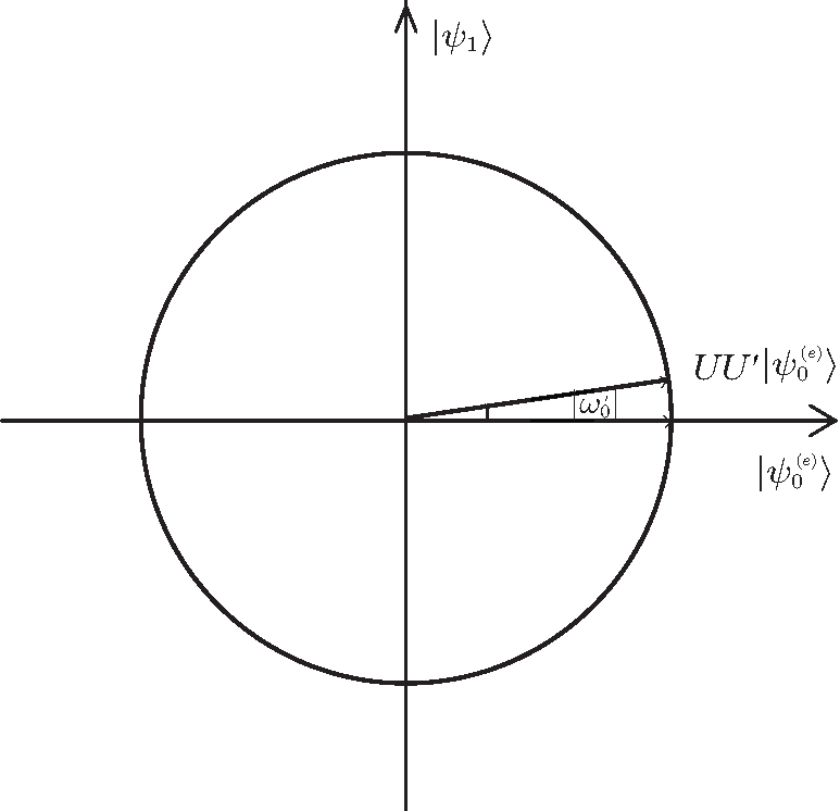 | Fig. 1. Each iteration of the algorithm UU′ can be viewed as a rotation in the plane composed of the initial state | ψ 0(e)〉 and the final state | ψ 1〉 . The rotation angle is  |
The model of the algorithm with phase errors can be built using the geometric description of the original algorithm. We assume a database size of 2n− 1. As the Grover operator imperfection in phase inversions of the algorithm is systematic, the explicit form of the inaccurate operator can be written as

where θ = π + δ and δ is a constant error. When δ = 0, the inaccurate operator degenerates to the original operator. The coin operator with errors can then be written as

The evolution operator becomes


Each iteration of the algorithm becomes 
First, we analyze the eigenvalue spectrum of 

k ≠ 0, k ≠ n. When k = 0, 


For the eigenvalue of 


According to Theorem 1 and Ref. [18], the random walk that introduces phase errors can also be collapsed onto a random walk on the line. To redefine the operator, where

the specific form of 
Expanding eigenvalues of 

When δ = 0 and n is replaced by n + 1, equation (30) becomes equal to Eq. (13). Then, we evaluate
obtaining

Similarly,
and
From Eqs. (32) and (34), it can be inferred that, when n is big enough, | ψ 0(e)〉 is an eigenvector of 

With the error increasing gradually, 

Expanding | ψ 0(e)〉 and | ψ 1〉 with 


where | γ 0〉 and | γ 1〉 are the normalized vectors orthogonal to 

we obtain
Similarly, evaluating 
Now, the algorithm with phase errors can be geometrically described using the expressions derived above. Applying the operator on the initial state | ψ 0(e)〉 successively t times, we get
where
which is determined by eigenvalues 

When δ = 0, 


The above analysis shows that when the algorithm has phase errors, the success rate of the algorithm and the required number of iterations will decrease.
The relationship between the size of the database, the phase error, the number of iterations, and the amplitude of the marked state was shown through the analysis described in the preceding section. We also analyzed the effects of the phase error on the algorithm. In this section, we will analyze the impact of phase errors on the success rate and the number of iterations by using numerical simulations, and demonstrate the quantitative relationship between the size of the database, the phase error, the number of iterations, and the success rate.
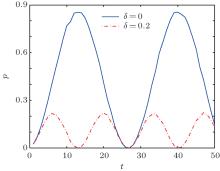
First, we simulate the relation between the number of iterations and the success rate when n = 8. We compare the two cases where δ = 0 and δ = 0.2, as shown in Fig. 2.
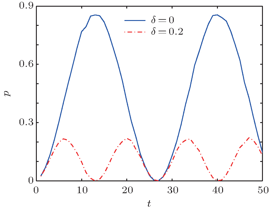 | Fig. 2. Relationship between the success rate of the algorithm p and the number of iterations t when n = 8. The solid line represents δ = 0.2 and the dotted line represents δ = 0. |
The solid line indicates that the algorithm without errors iterates 13 times to reach the maximum probability. The dotted line indicates that when the error is 0.2, the algorithm requires 6 iterations to reach the maximum probability, which is much smaller than the maximum probability obtained in the previous case. Both success rates change periodically with the number of iterations. The simulation results are consistent with the theoretical analysis in Subsection 4.2.
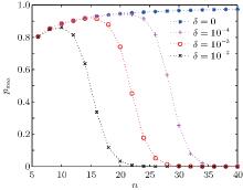
Next, we study the relationship between the maximum success rate of the algorithm, the database size, and the phase error. Each curve represents different phase errors, with δ = 0, δ = 10− 2, δ = 10− 3, and δ = 10− 4, as shown in Fig. 3.
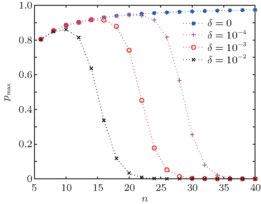 | Fig. 3. Maximum success rate of the algorithm pmax versus the scale of the database n with different phase errors. Different lines show results for different values of δ . |
Figure 3 shows that the maximum success rate increases with increasing database size. However, once it reaches a particular threshold, the value decreases exponentially. The larger the error, the smaller the database scale when the maximum success rate begins to decrease. With curve fitting, we obtain a relationship between the maximum success rate pmax, the size of the database 2n, and the phase error δ ,

p0 is the success rate of the algorithm without errors. It can be obtained from Section 4 that
Combining Eqs. (42) and (43), we obtain

It can be seen from Eqs. (44) that, before the search, to ensure the success rate of the algorithm, we need to predict the size of the phase error to limit the size of the database. For example, if the requirement of the success rate is not less than 0.5, the database size cannot be more than 3.8/δ 2.
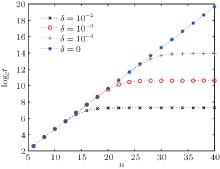
Next, we study the relationship between the iteration times required to reach the maximum success rate, the size of the database, and the phase error. The corresponding simulation results are shown in Fig. 4.
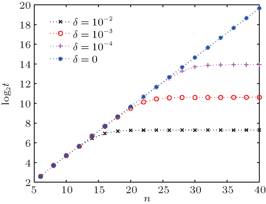 | Fig. 4. Scale of the required iteration times log2t versus scale of database n with different phase errors. The different lines show results for different values of δ . |
Figure 4 shows that the required number of iterations t0 increases with increasing database size. Beyond a particular threshold for a given error, the required number of iterations remains the same; this threshold database scale gets smaller as the errors become larger. Using curve fitting, we obtain the relationship between iteration times t0, the size of the database 2n, and the phase error δ ,

From the above analysis, it can be inferred that, when phase errors are present, the maximum success rate of the algorithm and the required number of iterations are the same as in the original algorithm as long as the database scale does not exceed a critical value, which suggests that this algorithm has tolerance to this sort of error. Comparing Fig. 3 with Fig. 4 for a given error level, we find that the corresponding database scale when pmax begins to decrease is smaller than that when t0 begins to remain constant; therefore, it is clear that pmax is more sensitive to the influence of the error. We define the value of n when pmax begins to decrease as the critical value. When pmax begins to decrease, we obtain the corresponding (δ , n) using numerical simulations. The expression relating the database scale n to the phase error δ is

Therefore, when the algorithm is in the presence of errors, the results are almost unaffected as long as the database scale satisfies the relation 
Now, we respectively obtain the expressions for maximum success rate pmax and the required iteration times t0 as a function of the phase error δ and the database size 2n. From the analysis of Subsection 4.2, the probability to obtain the marked state p is a periodic function, which can also be confirmed from Fig. 2. Thereby, making use of Eqs. (44) and (45), we obtain an expression for the database size 2n, the phase error δ , the number of iterations t, and the success rate p,
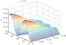
According to Eq. (47), for a given database size and expected error, we can calculate the number of iterations required to obtain a target success rate. This improves the efficiency of the algorithm, as shown in Fig. 5 for n = 8. When δ = 0 or δ = 0.2, the results are the same as those in Fig. 2.
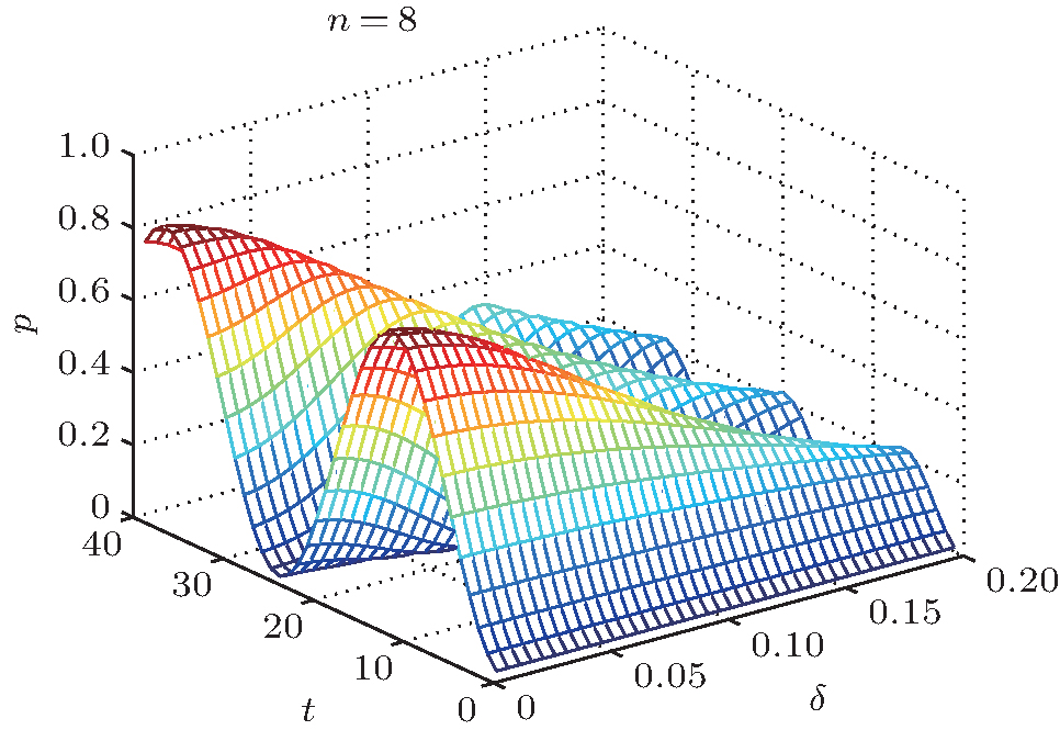 | Fig. 5. Three-dimensional graph of Eq. (47) when n = 8. The x axis shows the number of iterations t. The y axis is the phase error δ and the z axis is the success rate of the algorithm p. |
Finally, we make a simple comparison of robustness against phase errors between the optimized SKW algorithm and Grover’ s algorithm. Probability gap is defined as the probability difference between the marked state and the maximum rest state, [21] and is given by

In practice, as long as there is a sufficient probability gap, the probability of finding the marked state is much higher than other states at the end of the algorithm, and the algorithm is still successful. If the algorithmic probability gap variance is small regardless of the presence of errors, the robustness of the algorithm is strong; therefore, measuring the difference between probability gaps before and after the introduction of errors enables us to compare algorithmic robustness.
According to Ref. [20], the relationship between the database size, the phase error, and the maximum success rate is given in Grover’ s algorithm,

Therefore, the probability gap of Grover’ s algorithm is

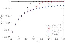
First, we simulate the probability gap for the optimized SKW algorithm Δ p1 with different phase errors. Figure 6 shows the result of this simulation. We then simulate the difference between the probability gaps Δ p1 − Δ p2, shown in Fig. 7.
The probability gap of the optimized SKW algorithm decreases exponentially with increase in errors, as shown in Fig. 6. However, for the same database scale, the difference between the probability gaps increases gradually, as shown in Fig. 7. These data indicate that the probability gap of Grover’ s algorithm decreases faster, proving that the optimized SKW algorithm is more robust.
 | Fig. 6. Probability gap of the optimized SKW algorithm Δ p1 versus the scale of the database n with different phase errors. The different lines show results for different values of δ . |
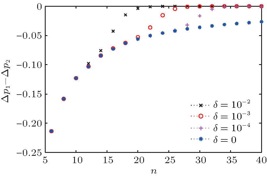 | Fig. 7. Difference between the probability gaps Δ p1 − Δ p2 versus the scale of the database n with different phase errors. The different lines show results for different values of δ . |
This study investigates the effects of systematic errors in phase inversions on the optimized SKW algorithm in detail. We first restate the optimized SKW as a geometric description, enabling the construction of the model of this algorithm with phase errors. Phase errors are shown to reduce both the number of iterations and the success rate of the algorithm through theoretical analysis and numerical simulations. Larger errors lead to a smaller maximum success rate of the algorithm and fewer number of required iterations. We derive relationships for both the maximum success rate of the algorithm and the required iteration times as a function of the phase error and the database size. Subsequently, we obtain a critical value for the database scale n. When 
| 1 |
|
| 2 |
|
| 3 |
|
| 4 |
|
| 5 |
|
| 6 |
|
| 7 |
|
| 8 |
|
| 9 |
|
| 10 |
|
| 11 |
|
| 12 |
|
| 13 |
|
| 14 |
|
| 15 |
|
| 16 |
|
| 17 |
|
| 18 |
|
| 19 |
|
| 20 | [Cited within:2] |
| 21 |
|