Typical spin– orbit coupling (SOC) of electrons in a solid state system is due to the relativistic effect. For instance, it can be derived from the Dirac equation of fermions by expanding in terms of the small parameter v/ c ≈ 0.01, which is the ratio of electron speed to light speed in solids. Therefore, the spin– orbit interaction is much weaker than the Coulomb interaction and is generally neglected in the study of condensed matter physics. However, it has been recently noticed that the SOC plays a crucial role in leading to the so-called topological insulating states in solids.^{[1, 2]} Consequently, it attracts many physicists’ attention. In particular, with successful realization of the synthetic gauge field in ultracold quantum gases, ^{[3– 7]} it is discovered that the spin– orbit coupling may also be important in determining the properties of these systems.^{[8– 26]} For example, the SOC can produce various new types of ground states, such as the stripes, the half-vortex phases in the Bose– Einstein condensates, and a bounded state, which is called Rashbon in the Fermi gases.^{[27– 29]} This makes research on SOC in ultracold gases vigorous.

In addition, ultracold gases in optical lattices have been used to simulate a wide range of condensed-matter phenomena, ^{[30, 31]} such as the Mott metal– insulator transition and the effects of strong correlation in the Hubbard model.^[32] As is known, at half filling, the low energy physics of these systems can indeed be described by an effective antiferromagnetic spin Hamiltonian in the deep Mott regime.^{[33– 36]} Therefore, the ground states are generally Neel ordered and the corresponding low-lying excitations are antiferromagnetic magnons.

Then, a question naturally arises: What effects will be induced if the SOC exists in ultracold gases loaded in an optical lattice? Recently, there has been considerable interest in exploring the intriguing physics in spin– orbit coupled optical lattices.^{[37– 49]} Many researchers have analyzed the phase diagrams of the spin– orbit coupled lattices in the deep Mott regime.^{[43– 47]} It was shown that one can derive an additional Dzyaloshinskii– Moriya (DM) type of super-exchange interaction^{[50, 51]} by using the second-order perturbation theory. Furthermore, by applying the classical Monte– Carlo simulations, several exotic spin textures, whose existences were previously explored in various solid state materials with the DM interaction, ^{[52– 54]} were also found in ultracold gases.

However, these investigations are not complete in theory. Indeed, up to now, the effects of spin fluctuations on the stabilities of the exotic spin textures in these phases have not been discussed yet. As is well known, strong spin fluctuations in low-dimensional systems can qualitatively change their phase diagrams outlined by the classical simulations. Therefore, one has to consider these fluctuations in order to determine the stability of each possible phase. In the following, we shall proceed to calculate the low-lying spectra of spin fluctuations in these phases. As a result, we are able to determine the parameter region in which each corresponding phase is stable against the spin fluctuations.

We implement the spin-wave method^{[55– 59]} to derive the global magnetic phase diagram of the super-exchange Hamiltonian. In particular, we calculate the spin-wave excitation spectra for the XY-ferromagnet phase, the spiral spin phase, and the spin vortex phase, whose existence has been studied by the previous classical Monte Carlo simulations.^{[43, 44]} We also discuss the stability of a novel phase, the so-called skyrmion crystal phase in bosonic ultracold gases. We show that the possible existing regions for the skyrmion crystal phase are greatly shrunk by the spin fluctuations. More precisely, we find that the spin excitation spectrum of the commensurate spiral spin phase has two minima, which are symmetrical with respect to the k_y axis in the momentum space. In addition, it possesses a gap. On the other hand, the spin fluctuations strongly destabilize the classical ground state of the skyrmion phase with the appearance of an imaginary part in the eigenfrequencies of spin excitations. Given that the above exotic spin configurations have also been discovered and attracted great interest, ^{[52– 54]} such features of the spin excitation spectra also provide insights into these spin phases.

This paper is organized as follows. In Section 2, we derive the effective super-exchange spin model for the systems of bosonic gases on a square optical lattice. In Section 3, we present the general formalism of the spin wave theory. Then, in Section 4, we analyze the phase diagram and the excitation spectrum of each above-mentioned phase in detail. Finally, in Section 5, we summarize our main results and discuss some related issues with experiments.

Let us consider a Bose gas loaded in a two-dimensional square optical lattice. The atoms are characterized by two nearly-degenerate states, which are produced by a hyper-fine interaction. In the following, for convenience, we shall use the language of (pseudo)-spin to describe the local occupancy of these states. Furthermore, we take the synthetic spin– orbit interaction into consideration. Then, the Hamiltonian of the bosonic gas can be written as

Here denotes the boson annihilation (creation) operator, which annihilates (creates) a boson of (pseudo)-spin σ = ↑ , ↓ at lattice site i. In a compact form, these operators can be rewritten as and its Hermitian conjugate ψ _i. The first term of H describes the hopping process of bosons between a pair of nearest-neighbor lattice sites i and j. The corresponding hopping matrices are given by , where A = (α σ _y, β σ _x, 0) is a non-Abelian gauge field with σ _x and σ _y being the Pauli matrices.^{[43, 44, 60]} In fact, if we let β = − α , then A = (α σ _y, − α σ _x, 0) is the gauge field giving rise to the well-known Rashba SOC. The diagonal part of the hopping matrices represents the spin-conserved tunneling, while the off-diagonal part is for the spin-flipped tunneling of bosons between lattice sites i and j. The second term in the Hamiltonian denotes the contact interaction between bosons. In general, the intra-species interaction strengths can be different. However, we assume them to be equal in the following discussion. More precisely, we set U_{↑ ↑} = U_{↓ ↓} = U. Similarly, we choose the inter-species interaction U_{↑ ↓} = U_{↓ ↑} ≡ λ U with λ > 0 being a dimensionless parameter.

As is well known, the filling factor of bosons is also an important parameter to determine the properties of ultracold gases in an optical lattice. In the following, we shall only consider the case of one boson per site on average. Now, we can perform the standard Schrieffer– Wolf transformation H_eff = e^iSH e^{− iS[61]} to the Hamiltonian in the large-U limit U_{σ σ ′} ≫ t. It produces an effective Hamiltonian

which captures the low-energy physics of the original system.^{[43, 44, 62]} Here, are the spin operators of bosons at lattice site i. In terms of the boson operators a_iσ and , they can be written as , , and . In Eq. (2), the first summation is a Heisenberg type of Hamiltonian and the second summation represents the so-called Dzyaloshinskii– Moriya superexchange interaction. The corresponding coupling constants are given in Table 1.

Table 1.

Table 1.

Table 1. Exchange couplings for the Heisenberg term and Dδ for the DM superexchange interaction in the effective Hamiltonian.

Table 1. Exchange couplings for the Heisenberg term and Dδ for the DM superexchange interaction in the effective Hamiltonian.

We would like to emphasize that these interactions favor qualitatively different types of spin orders. In fact, the Heisenberg Hamiltonian gives either the ferromagnetic or the anti-ferromagnetic ordering, while the DM interaction makes the spiral spin ordering possible. In other words, there exists a competition between them. Consequently, their interplay may drive the system to various exotic phases. In the following, we shall first determine the possible existence of several phases in the system, and then analyze their stabilities by applying the spin-wave theory.

Fig. 1.

	Figure Option ViewDownloadNew Window
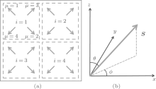
	Fig. 1. (a) Spin configuration of the 2× 2 spin vortex phase, where i denotes the magnetic primitive cell and μ is the sublattice index. (b) The spin is rotated from the z axis to a new direction (θ , ϕ ) in the spin-wave theory.

In the previous works, some authors have explored the classical ground states of Hamiltonian (2) by the classical Monte Carlo simulations.^{[43, 44]} They showed that the classical ground states of this system support a variety of phases, such as the XY-ferromagnetic (XY-FM) phase, the longitudinal ferromagnetic (Z-FM) and antiferromagnetic (Z-AFM) phases, the spiral spin phase, the 3× 3 skyrmion crystal (SkX) phase, and the 2× 2 spin vortex (VX) phase, as the coupling constants of the Hamiltonian are changed. However, they did not consider the stabilities of these phases. In order to address this issue, one has to take the strong spin fluctuations of the system into consideration, as we will do in the following.

To start with, we shall first calculate the ground state energy of each above-mentioned phase in some specified regions of parameters by the mean-field theory and see if the previous phase diagram can be re-established. Then, we compute the second-order correction to the energies of these phases. This correction is due to the spin-wave excitations. In some cases, it can render the phase derived by the classical methods invalid. More precisely, as we shall show in the following, the excitation spectrum of a specified phase may develop an imaginary part and hence, becomes a complex function of momentum in some parameter regions. It implies that the presumed phase is actually unstable against the spin fluctuations in these regions. To illustrate the procedure, let us take the 2× 2 VX phase for example.

In the first step, we perform the following transformation:

where i denotes the spin primitive cell of the specified phase and μ is the sublattice index, as shown in Fig. 1(a). The matrix  _μ reads

It represents the rotation of each spin in the Hamiltonian from the local z axis to a new direction (θ , ϕ ), as shown in Fig. 1(b).

Next, we apply the Holstein– Primakoff transformation^[63] by substituting the spin operators , , into the effective Hamiltonian. Consequently, we obtain H_eff ≃ H₀ + H₂. Here, H₀ denotes the mean-field energy for a specific phase and H₂ is the spin-wave Hamiltonian, which describes the spin fluctuation in the system. Let N be the total number of lattice sites, the mean-field energy H₀ can be written as

Here, the spin angles θ _μ and ϕ _μ are determined by the spin configurations of the specified mean-field ground state. For example, in the 2× 2 VX phase, we have θ ₁ = θ ₂ = θ ₃ = θ ₄ = π / 2, ϕ ₁ = 3π / 4, ϕ ₂ = 7π / 4, ϕ ₃ = π / 4, and ϕ ₄ = 5π / 4. In addition, (μ , ν ) and (α , β ) denote two pairs of nearest-neighbor sites in the primitive cell along the and axes, respectively. With the same notations, we obtain the following spin-wave interaction terms

by keeping only the terms of two-boson operators in the expansion of the transformed effective Hamiltonian. Here, W_μ , M_{μ , μ ′} , and N_{μ , μ ′} are the coefficient matrices depending on the mean-field spin configuration. The explicit expressions of the matrices are given in Appendix A. Then, by using the Fourier transformation, we are able to rewrite H₂ as

where are boson operators in the momentum space, and the Hamiltonian matrix H_MN is given in Appendix A. Now, we apply the Bogoliubov transformation to the effective Hamiltonian H₂. Due to the bosonic commutation relation, the transformation matrix must be canonical, i.e., relation should hold, where

Furthermore, after substituting the Bogoliubov transformation into Eq. (6), we determine the transformation matrix by requiring that the Hamiltonian be diagonalized by it. In other words, the matrix product should be a diagonal matrix. With the canonical constraint , this condition can be put into an equivalent form

Consequently, by diagonalizing H_MNΛ with an invertible matrix , we can derive the spin excitation spectrum ω _{k, μ} , and then discuss the stability of the 2× 2 VX phase by checking whether the obtained checking excitation spectral function is complex.

In the following section, we will study the possible existence and stability of the XY-FM phase, Z-FM phase, Z-AFM phase, spiral spin phase, 3× 3 SkX phase, and 2× 2 VX phase in ultracold gases on a square optical lattice by the above-outlined procedure. As is shown below, although this procedure can be easily applied to most of these phases, it is rather involved for the 3× 3 skyrmion crystal phase. The main difficulty is due to the complicated spin configuration of this phase. It contains nine sublattices. In other words, according to the local spin orientations in the 3× 3 skyrmion phase, the whole lattice can be divided into nine separate sublattices. In each of them, all the localized spins point in a specified direction. A primitive spin cell of this phase is shown in Fig. 2(b).

First, we compute the ground-state energy H₀ for each possible spin configuration listed in the last section and determine the phase diagram by choosing the lowest energy configurations in different parameter regions. Then, we compare our results with the previous ones derived by the classical Monte Carlo calculations. Our phase diagram is shown by the solid lines in Fig. 2(a). It is in good agreement with the Monte– Carlo simulations given in Ref. [43].

Next, we calculate the spin-wave excitation spectrum of each phase and see if it is stable against the spin fluctuations. In fact, we find that the Z-AFM and 2× 2 VX phases are stable. However, the 3× 3 SkX phase is pronouncedly affected by the spin fluctuations. Actually, in two parameter regions, i.e., the white areas in Fig. 2(a), the spin-wave excitation spectral functions have imaginary parts and hence, render the corresponding phases unstable. On the left side of the commensurate 4× 1 spiral phase, the unstable parameter region implies the emergence of other commensurate spiral orders or incommensurate spiral phases. While the right unstable parameter region may support new states, which need to be further investigated in future. Now, let us analyze the spin excitation spectrum of each phase in a more detailed manner.

Fig. 2.

	Figure Option ViewDownloadNew Window
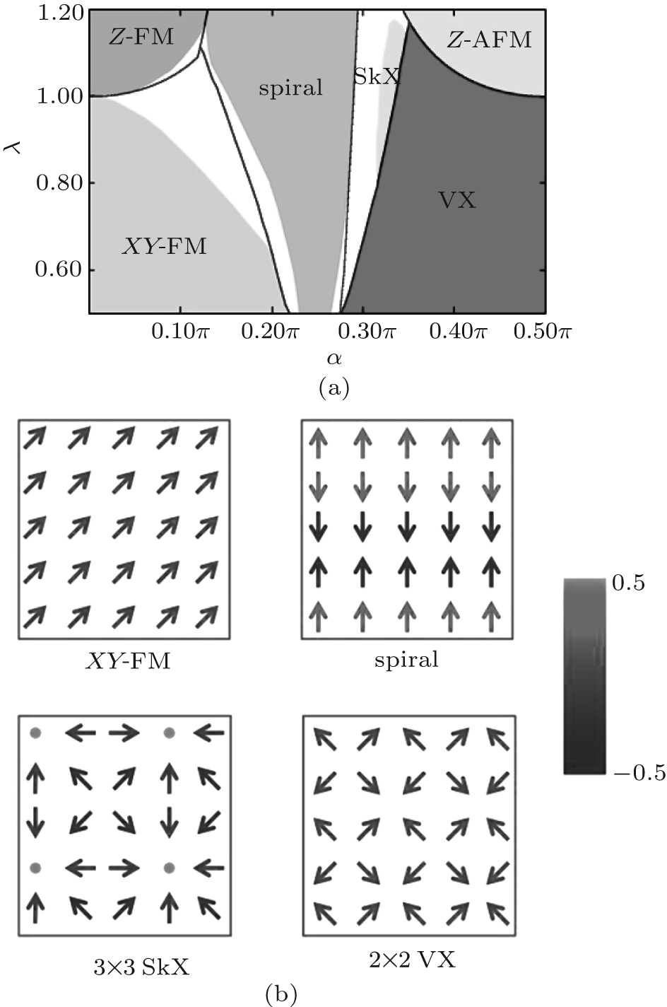	Fig. 2. (a) Phase diagram in the Mott insulating regime. The solid lines are the mean-field results. The filled areas with colors are the stable regions, while the white areas are the unstable ones under the spin-wave fluctuations. (b) Spin configurations of the XY-FM, commensurate 4× 1 spiral spin, 3× 3 SkX, and 2× 2 VX phases.

We first consider the weak spin– orbit coupling regime in which the parameter α in Table 1 is small. In this case, the Heisenberg interaction in Hamiltonian (2) is dominant and the DM interaction can be treated as a perturbation. In particular, if we set α = 0, the effective Hamiltonian becomes the standard ferromagnetic XXZ model on a two-dimensional square lattice.^[64] The phase diagram of this model is for λ < 1, and all the spins are aligned in the XY plane. More precisely, the system is in the XY-FM phase. In this phase, the Holstein– Primakoff transformation can be easily applied. A direct calculation yields for its spin excitation spectrum, in which and a is the lattice constant. Obviously, the excitation spectrum is gapless with a linear dispersion near | k| ∼ 0, which corresponds to the Goldstone modes in the XY-ferromagnets. On the other hand, for λ > 1, the system is in the Z-FM phase. The spin excitation spectrum of this phase is given by , which has a spin gap at Δ = J(2λ − 2). Finally, λ = 1 is the so-called Heisenberg point at which the model becomes the isotropic Heisenberg ferromagnet. It has a gapless quadratic excitation spectrum, which is shown in Fig. 3.

Fig. 3.

	Figure Option ViewDownloadNew Window
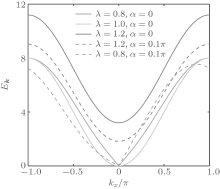
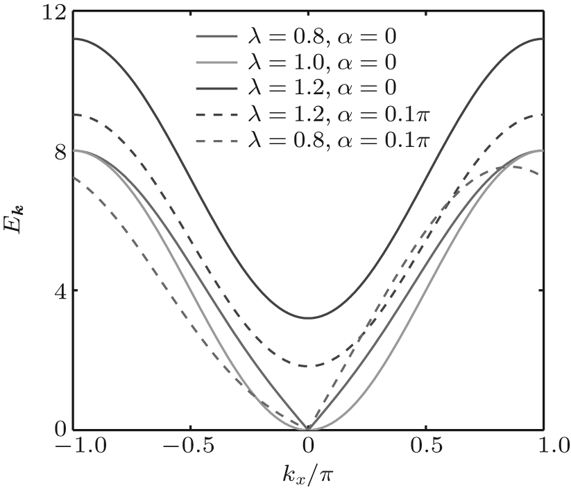	Fig. 3. The excitation spectra for the XY-FM (λ = 0.8), Z-FM (λ = 1.5), and Heisenberg ferromagnetic (λ = 1) phases. Solid and dashed lines are for α = 0 and α = 0.1π , respectively.

Next, we take the effect of the DM interaction into consideration. We find that the excitation spectrum remains gapless and linear near ∣ k∣ ∼ 0 for the XY-FM phase. However, it becomes asymmetric with respect to k_x = 0, as shown by the dashed line of λ = 0.8 and α = 0.1π in Fig. 3. A similar dispersion occurs along the k_y axis. In the meantime, the gap of the Z-FM phase is decreased upon the increased strength of the SOC. However, both the spin excitation spectra of the XY-FM and Z-FM phases will become imaginary as the SOC strength α is further increased. It indicates that these phases are destabilized. This region of parameters is characterized by the white area on the left side of the spiral phase in Fig. 2(a).

In the middle region of Fig. 2(a), the DM interaction is strong, comparing with the Heisenberg interaction. The competition between these interactions leads to a spiral spin phase. To determine the stability of this phase, we consider a commensurate 4× 1 periodic structure with all the spins lying in the z– y plane. Notice that, in this configuration, the angles θ _i between the spins and the z axis are specified by θ ₁ = θ ₂, θ ₃ = θ ₄, and θ ₁ + θ ₃ = π .

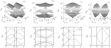
Then, we calculate the excitation spectrum of this phase by the spin-wave analysis. Our results are shown in Figs. 4(a) and 4(e). One can easily see that there exists a spin gap in the diagram. In other words, the Goldstone mode is absent in this phase. Moreover, the gap has two symmetric minima at (± k₀, 0), as shown in Fig. 4(a). It is due to the fact that the spin configuration of the spiral spin phase is symmetric with respect to the y axis. By varying parameter α , we find that the energy gap gradually closes as the DM interaction increases and the excitation spectrum becomes linear in the vicinity of these minimal points. At the same time, the 4× 1 periodic structure becomes unstable. It suggests the emergence of other commensurate spiral orders or incommensurate spiral phases.

Fig. 4.

	Figure Option ViewDownloadNew Window
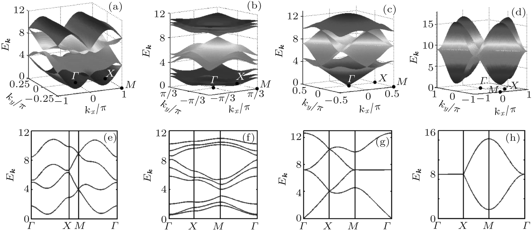	Fig. 4. The excitation spectra for (a), (e) 4× 1 spiral spin phase (λ = 0.8, α = 0.24π ), (b), (f) 3× 3 skyrmion crystal phase (λ = 0.9, α = 0.32π ), (c), (g) 2× 2 spin vortex phase (λ = 0.8, α = 0.4π ), and (d), (h) Z-AFM (λ = 1.2, α = 0.4π ) phase.

Next, let us consider the large spin– orbit coupling regime around α = π /2, in which the spin-conserved hopping of particles is suppressed. The Wilson loop which is characterized by is reduced to a marginally abelian one with | W| = 2.^[60] In this situation, the Heisenberg interaction is dominant and the spin configuration is determined by a uniform antiferromagnetic interaction in the z direction plus anisotropic spin-interactions in x and y directions. When parameter λ < 1, the spin interaction in the xy plane is stronger. Therefore, the system has a co-planar magnetic order. On the other hand, since the spin interaction is antiferromagnetic in the x direction but ferromagnetic in the y direction, the classical ground state of the system becomes a 2× 2 vortex crystal. Further analysis yields the spin-wave spectrum of this phase, as shown in Figs. 4(c) and 4(g). We find that it has no gap and is linear in the vicinity of the minimum Γ point. In contrast, for λ > 1, the system enters the Z-AFM phase. Its excitation spectrum is shown in Figs. 4(d) and 4(h). Now, energy gaps open up at momenta (± π , 0) and (0, ± π ).

Finally, we study the 3× 3 skyrmion crystal phase, which is located in the phase diagram between the 4× 1 spiral spin phase and the 2× 2 VX phase. As is mentioned at the end of Section 3, the spin configuration of this phase consists of nine sublattices, which are characterized by an up-spin at the center and others lying in the xy plane. By the spin-wave theory, we calculate its spin excitation spectrum. Our results are shown in Figs. 4(b) and 4(f). Obviously, the spectrum also has an energy gap. Interestingly, we find that the spin fluctuations dramatically destabilize this classical ground state and make the skyrmion crystal phase unstable in part of the classical phase diagram determined by the Monte Carlo simulations, ^[43] where the eigenfrequencies of spin excitations exhibit an imaginary part. It may imply the appearance of a novel state in the concerned region. However, more specific description on the possible new states in this regime is beyond the current spin-wave analysis, and one may use more sophisticated unbiased quantum Monte– Carlo simulations.

We study the exotic magnetic phases of two-component Bose gases with spin– orbit coupling on a deep square optical lattice by using the spin-wave theory. In particular, we systematically investigate the spin-wave excitation spectra for the XY-ferromagnet, spiral spin, spin vortex, and skyrmion crystal phases. We find that while the excitation spectrum of the vortex crystal phase has no gap and is linear in the vicinity of the center of the Brillouin zone, the spectra of the commensurate spiral spin phase and the skyrmion crystal phase possess energy gaps. We also discuss the stability of the novel skyrmion crystal phase and show that the possible existing regions for the skyrmion crystal phase are greatly shrunk by the spin-wave excitations. In Ref. [44], several methods for detecting spin textures in the Mott insulator phase have been proposed, such as noise correlations in time-of-flight (TOF) images and optical Bragg scattering. Finally, we would like to emphasize that similar spin textures, which are discussed in the present work, can also be induced by the DM type of interactions in some solid state materials. Therefore, we believe that the current investigation should provide further insights for the study of these materials.