Figure  1 shows a general distributed recoverable computational platform developed according to the ROBUS communication system. This platform is composed of N controller processing elements (CPEs), M redundancy management units (RMUs), bus interface units (BIUs), and one I/O PE. The functions of each unit are consistent with those in the previous work. In the present paper, CPEs are used to calculate the updates of control law in the sample period, and RMUs are used to coordinate the communications between the PEs, which guarantees to provide full and reliable messages. BIUs provide the interface between PEs and the whole communication system. I/O PE acts as an input– output interface to the actuators. In practical application, the processing units, CPEs and RMUs, are off-the-shelf devices; more details about the hardware implementation can be found in Refs.  [12], [13], and [21]. This part has been further studied in Refs.  [6] and [7]. In the present paper, analyses are based on several assumptions that are stated below.

The processes discussed in this paper are all binary random variables such as the upset processes, θ _i(k) and υ _ij(k). That is, when the random process is injected by an upset, ‘ 1’ will be taken and ‘ 0’ otherwise. All the CPE-BIU outputs, z_i(k), represent the state of the corresponding CPE at time k. Similarly, when z_i(k) is taken to be ‘ 0’ , the PE works properly at the time k, then it will present the correct update at that instant to the control law. Or it is upset and could not transmit a correct update to the control law. Each CPE is functioning with disturbance input θ _i(k) abiding by the state transition table given in Table  1.

Fig.  1.

	Figure Option ViewDownloadNew Window
	Fig.  1. A general N CPEs × M RMUs distributed computing platform topology based on ROBUS with digital upset injections.

Table 1.

Table 1.

Table 1. State transition table for the i-th CPE. CPE state zi(k) CPE upset θ i(k) CPE next state zi(k + 1) 0 0 0 0 1 1 1 0 0 1 1 1

Table 1. State transition table for the i-th CPE.

The same rule is also implemented on the inner channels of each RMU, where ẑ _ij represents the state of the channel i of the RMUj. ẑ _ij is subject to upsets specifically from the disturbance input υ _ij. Table  2 shows the state transition table used in the channel i of the RMU j. Correspondingly, when the output of a channel is ‘ 1’ , data from the associated CPE could not be reliably transmitted to I/O PE. The logics working on output of the channel ij, ŷ _ij(k) is operated as Logical OR where z_i(k) and ẑ _ij(k) determine the outputs. That means that if and only if (iff) the CPE and the RMU are both not injected by upset at time k, an update for the control law is available in this channel at this instant. Logical AND will be applied to I/O PE fed by all outputs of the communication channels. In this situation, if the I/O PE output z_υ (k) = 1, there is no control update for the closed-loop system. That, then, implies that the system must operate in the upset mode only when the next proper update at the (k + 1)-th sample is coming. Otherwise, the system will operate in a nominal mode. This explanation is consistent with those in Refs.  [6] and [7].

Table 2.

Table 2.

Table 2. State transition table for the channel i of RMU i. RMU state ẑ ij(k) RMU upset υ ij(k) RMU next state ẑ ij(k + 1) 0 0 0 0 1 1 1 0 0 1 1 1

Table 2. State transition table for the channel i of RMU i.

This paper employs a switched jump linear system to model the dynamics of the flight closed-loop system in the form of

The paper will analyze the performance degradation of the control system and the system stability when the stochastic process z_υ (k) is a general Markov process, an IID process with Markov format or an IID process.

As stated above, z_υ is a binary random variable and z_υ (k) is a stochastic process. Therefore, when z_υ takes ‘ 0’ and ‘ 1’ , the system is operating in nominal and upset modes. The corresponding nominal and upset state space models are represented by (A₀, B₀, C₀) and (A₁, B₁, C₁), respectively. The methods developed in this paper will be applied to a Boeing 737 control system model. The nominal and upset modes of the control system under consideration are both eighth-order realization. The paper uses the models from Ref.  [10] which provides the specific details about state space models. The purpose of performance analysis in this paper will focus on the altitude output variable. The state space models also include Dryden wind gust spectral shaping filters.^{[10, 11]} Since the system switches between normal and abnormal conditions, an error system shown in Fig.  2 is formed in order to evaluate the performance degradation when the system is subject to harsh environments. From the closed-loop system perspectives with Fig.  3, the input w(k), in fact, drives the shaping filters. Process noise generated by the filter will then be injected into the control-loop. In the event of no upsets subject to the control computer, the system will be operating in the nominal mode, then the generated tracking performance is acceptable. Once the nominal system is interrupted by an upset, the nominal system control law will be affected, then another different control law will replace the original one. The corresponding performance degradation is obvious. Therefore, the error system as shown in Fig.  2 is suited to analyze this degradation. Two copies of Eq.  (1) with the same input w(k) form an error system. One copy works as the reference system. This system is always operating in the nominal mode and will never switch to the upset mode. However, another copy works as the upset system switched by the upset switching signal z_υ (k). Therefore, there is a difference between their respective outputs, and the output error signal, y_e(k), could characterize the numerical difference.

Fig.  2.

	Figure Option ViewDownloadNew Window
	Fig.  2. Error system used for the performance analysis.

Fig.  3.

	Figure Option ViewDownloadNew Window
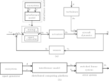
	Fig.  3. Complete performance model for the digital control system: (a) the complete configuration and (b) the concise configuration.

The main difficulty in analyzing the performance for the proposed method in this paper is that the method should be workable in the overall performance model structure including three subsystems as shown in Fig.  3. It comprises the computing platform shown in Fig.  1 and the error system shown in Fig.  2, and the upset generator producing disturbance process from the exosystem. Figure  3(a) is the complete overall configuration; figure  3(b) is the concise version. These upset processes are injected in the distributed computing platform called the interference model. The difference in the flight control system performance can be observed: the closed-loop error system is driven by the output of the interference model. The numerical evaluation of performance of interest uses the mean power of the output tracking error

If the error system is mean-square stable, the limit of the mean power exists. In this paper, J_{w, e} is described as a function of the design choices of N, M, the transition probability matrices of θ _i(k) and υ _ij(k), and dynamics of the flight control systems. Therefore, this design and the index of J_{w, e} are used to characterize the quality degradation of the system performance when the system is subject to upsets.

This paper considers that upset processes, θ _i(k) and υ _ij(k) are HMCs. Even though z_i(k) is a delayed version of θ _i(k), and ẑ _ij(k) is a delayed υ _ij(k), in general, z_υ (k) could not be of Markov.^[22] Then the paper derives the mean square performance metric of J_{w, e} from Ref.  [10]. Therefore, joint theorems are employed to generate an alternative but equivalent process which acts as the switching signal to drive the error system as shown in Fig.  2.

Definition 1ϕ , the structure function, is a memoryless, binary-valued mapping as shown in Fig.  4. This mapping is ϕ : {0, 1}^{N + M} → {0, 1} given by

Fig.  4.

	Figure Option ViewDownloadNew Window
	Fig.  4. Alternative conceptual schematic diagram for the computing platform with Markov upset processes.

Lamma 1 The binary random process z_υ (k) defined in Fig.  4 satisfies the identity

Proof It is evident from Fig.  1 and the assumptions (i), (iv), and (v) that

From the distributivity property of Boolean algebra and the properties between z_i(k), ẑ _ij(k), and θ _i(k), υ _ij(k), it follows that

This proves the lemma.

Lemma 2^{[23, 24]} Let θ _i(k) and υ _ij(k) be independent HMCs in state space {0, 1} with the transition probability matrices Π _{θ i} and Π υ _ij, respectively, for i = 1, … , N′ and j = 1, … , M′ , then the joint process u≜ (θ (k), υ (k)) will be an HMC with transition probability matrix

and state probability vector

where ⊗ denotes the Kronecker product and N′ , M′ represent the numbers of the processing units subject to upsets. When processes θ _i(k) and υ _ij(k) satisfy these properties, the joint process ū (k) is irreducible and aperiodic. The detailed proof can be found in Ref.  [23].

Even though z_υ (k) is not always a Markov chain, ^{[10, 23]} the joint process described below is always known as the Markov process.

Theorem 1^{[23, 24]} Let θ _i(k) and υ _ij(k) be independent HMCs in state space {0, 1} with the transition probability matrices Π _{θ i} and Π _{υ ij}, respectively, for i = 1, … , N′ and j = 1, … , M′ . Define z_υ (k) = ϕ (θ _i(k), υ _ij(k)) and the joint process, ū (k) = (θ (k), υ (k)), then a new joint process

will be an HMC process; therefore, its state space can be reduced to a proper subset of {0, 1}^{N′ + M′ + 1}. Equivalently, transition probability matrix of the joint process ρ (k), Π _ρ , is Π _ū . When θ _i(k) and υ _ij(k) are irreducible and periodic with invariant distributions, the joint process ρ (k) is ergodic. That means that ρ (k) is modeled to be equivalent to z_υ (k) in Eq.  (1) for each state vector (ū , z_υ ) according to the model equivalence definition introduced in Ref.  [25]. Therefore, the HMC ρ (k) can substitute for z_υ (k) to drive the switched linear model.

The main contribution of this paper is to specifically propose the performance index analysis of J_{w, e} when the substituted switching signal ρ (k) is a homogeneous first-order or zero-order Markov chain. Since all the upset processes are directly injected into the system, the estimation method becomes much more complex, and this is also a big difference from the previous work. Some specific definitions and theorems about the performance index of J_{w, e} are applied to the error system as shown in Fig.  2 by using switching signal ρ (k).

Consider an n-dimensional jump-linear error system:

where A_{e, ρ} = diag(A_ρ , A₀), , and C_{e, ρ} = [C_ρ , − C₀]. The process ρ (k) has states labeled by the symbols l = 0, 1, … , (l₀ + l₁). Here, l₀ and l₁ represent the numbers of “ 0” and “ 1” in ρ , respectively.

The following Theorems 2 and 3 are derived from Ref.  [10].

Theorem 2 The Markov jump-linear system (2) is MSS iff r_σ (A₂) < 1, where

where Π is the transition probability matrix for ρ (k), and r_σ (· ) is the spectral radius. This is derived from Ref.  [16].

Theorem 3 For the MSS Markov jump-linear system  (2), where ρ (k) is aperiodic and ergodic, if x₀ = 0, and w(k) and ρ (k) are independent, then

where C = (C₀, C₁, … , C_l0 + _{l1 − 1}) is an l₀ + l₁-tuple with

with and denoting the inverse column stacking operator for the column array from ln to (l + 1)n − 1.

Theorem 4 Consider an N CPEs × M RMUs computing platform topology as shown in Fig.  1, where N′ CPEs and M′ RMUs are subject to upsets (N′ ≤ N, M′ ≤ M). Let each θ _i(k) random process have a certain probability p_θ := P{θ _i(k) = 1}, and likewise, let each υ _ij(k) random process have a certain p_υ : = P{υ _ij(k) = 1}. Suppose that n_s CPEs or m_s RMUs have the same upset probabilities p_{θ s} and p_{υ s}, (∑ n_s = N′ , ∑ m_s = M′ , s = 1, 2… ). Suppose that the random processes, θ _i(k) and υ _ij(k), are mutually independent, and they are independent of the initial conditions of z_i(0) and ẑ _ij(0), then the stationary probability will be characterized by

Proof According to the computer platform configuration shown in Fig.  1, assumptions and the state transition tables shown in Tables  1 and 2, we have

It is known that the voter is a Logic AND of inputs, and state random variables z_i(k) are independent, then

Since the output of the ij-th channel, ŷ _ij(k), is used as Logic OR of z_i(k) and ẑ _ij(k), it is obvious that

Therefore,

It is claimed that {z_i(k = 0} and are independent for any fixed i and k, therefore,

Since random process z_i(k) is a delayed version of random process θ _i(k), and random process ẑ _ij(k) is a delayed version of random process υ _ij(k), then by substituting these identities into the above equation, equation  (2) can be yielded. In addition, θ _i(k) and υ _ij(k) can be IID and are independent of the initial conditions. Apply De Morgan’ s Law to Eq.  (2), then we will have

Since the upset probabilities for CPEs or RMUs can be varied or part of them are the same, therefore, the identity shown above can be expressed in a concise way as follows:

where n_s and m_s represent the numbers of upset processes injected into CPEs and RMUs with the same upset probabilities, respectively. Therefore, the identity  (3) is obtained.

It is known that z_υ (k) is a two-state IID process and switches the jump linear system, therefore, equation  (1) can be converted into the following format

Like Theorem 2, the A_{e, 2} matrix becomes

Correspondingly, Theorem 3 can be specifically changed into

where C = (C₀, C₁) is a 2-tuple with

with and denoting the inverse column stacking operator for the column array from ln to (l + 1)n − 1.

Theoretical performance analysis described by Eq.  (2) is employed in the Boeing 737 flight control system with the CPEs and RMUs subject to independent Markov upsets. As shown in Fig.  4, independent Markov upsets are jointed, and the jointed transition probability matrix is injected to the ϕ function. Therefore, the new joint process, the switching signal ρ (k), is the HMC process according to Lemma 2 and Theorem 1. Tracking performance error evaluation can be estimated by Theorem 3, and the stability analysis method is also proposed. The specific example is shown below. Theoretical estimation examples for the upset processes with general Markov chains, IID processes of the Markov format, and individual IID processes are analyzed in detail below.

Example 1 Consider a 2CPEs × 2 RMUs computing platform topology where two CPEs and one RMU are subject to independent Markov digital upsets. Suppose that the HMC’ s transition probability matrices for θ _i(k) and υ _ij(k) are given. Some of the matrices are estimated based on the analysis of experimental data calculated by Eq.  (3).^[8] The data are collected from the experiments conducted under the 121.15-MHz frequency and 140-V/m field strength electromagnetic environment will be partly employed in this example, and the transition probability matrix estimated from the experimental result is

Others are randomly chosen and shown below

Table  3 provides a state table for the joint process. It is evident that ρ (k) has 16 states from Table  3, therefore, the corresponding transition probability matrix of the joint process ρ (k), and state probability vector of ρ (k) can be calculated by Lemma 2 and Theorem 1 as follows:

The corresponding A_{e, 2} matrix is

Using Theorem 3 in the calculations above, the theoretical estimation of performance index of J_{w, e} is 0.5928. Simultaneously, the error system for this example is stable since the spectral radius of the matrix A_{e, 2} is less than one.

Next, since the IDD process is a zero-order HMC process, then we take an IID case with the Markov format as an example.

Table 3.

Table 3.

Table 3. State table for the 2 CPEs × 2 RMUs computing platform when two CPEs and one RMU are injected by digital independent Markov upsets at time k. θ 1 θ 2 υ 11 υ 21 υ 12 υ 22 zυ ρ 0 0 0 0 0 0 0 ρ 1: (0 0 0 0 0 0 0 ) 0 0 0 1 0 0 0 ρ : (0 0 0 1 0 0 0 ) 0 0 1 0 0 0 0 ρ 3: (0 0 1 0 0 0 0 ) 0 0 1 1 0 0 0 ρ 4: (0 0 1 1 0 0 0 ) 0 1 0 0 0 0 0 ρ 5: (0 1 0 0 0 0 0 ) 0 1 0 1 0 0 0 ρ 6: (0 1 0 1 0 0 0 ) 0 1 1 0 0 0 0 ρ 7: (0 1 1 0 0 0 0 ) 0 1 1 1 0 0 0 ρ 8: (0 1 1 1 0 0 0 ) 1 0 0 0 0 0 0 ρ 9: (1 0 0 0 0 0 0 ) 1 0 0 1 0 0 0 ρ 10: (1 0 0 1 0 0 0 ) 1 0 1 0 0 0 0 ρ 11: (1 0 1 0 0 0 0 ) 1 0 1 1 0 0 0 ρ 12: (1 0 1 1 0 0 0) 1 1 0 0 0 0 1 ρ 13: (1 1 0 0 0 0 1) 1 1 0 1 0 0 1 ρ 14: (1 1 0 1 0 0 1) 1 1 1 0 0 0 1 ρ 15: (1 1 1 0 0 0 1) 1 1 1 1 0 0 1 ρ 16: (1 1 1 1 0 0 1)

Table 3. State table for the 2 CPEs × 2 RMUs computing platform when two CPEs and one RMU are injected by digital independent Markov upsets at time k.

Example 2 Consider a 3CPEs × 2 RMUs computing platform topology where three CPEs are subject to IID digital upsets under the electromagnetic environment of 133.35-MHz frequency and 210-V/m field strength. In addition, in this example the Markov format is used to describe IID upset processes. Suppose that θ _i(k) and υ _ij(k) are IID processes, transition probability matrices for θ _i(k) and υ _ij(k) with IID properties will be

Following the analysis procedure in Example 1, Π _ρ , π _ρ (0), and the corresponding A_{e, 2} matrix are calculated according to Table  4 by

and

Then theoretical performance estimation of J_{w, e} is 6.5399 × 10^-5.

Table  4.

Table  4.

Table  4. State table for the 3 CPEs × 2 RMUs computing platform when three CPEs are injected by IID digital upsets with Markov format at time k. θ 1 θ 2 θ 3 υ 11 υ 21 υ 31 υ 12 υ 22 υ 32 zυ ρ 0 0 0 0 0 0 0 0 0 0 ρ 1: (0 0 0 0 0 0 0 0 0 0) 0 0 1 0 0 0 0 0 0 0 ρ 2: (0 0 1 0 0 0 0 0 0 0) 0 1 0 0 0 0 0 0 0 0 ρ 3: (0 1 0 0 0 0 0 0 0 0) 0 1 1 0 0 0 0 0 0 0 ρ 4: (0 1 1 0 0 0 0 0 0 0) 1 0 0 0 0 0 0 0 0 0 ρ 5: (1 0 0 0 0 0 0 0 0 0) 1 0 1 0 0 0 0 0 0 0 ρ 6: (1 0 1 0 0 0 0 0 0 0) 1 1 0 0 0 0 0 0 0 0 ρ 7: (1 1 0 0 0 0 0 0 0 0) 1 1 1 0 0 0 0 0 0 1 ρ 8: (1 1 1 0 0 0 0 0 0 1)

Table  4. State table for the 3 CPEs × 2 RMUs computing platform when three CPEs are injected by IID digital upsets with Markov format at time k.

Next, when θ _i(k) and υ _ij(k) are IID processes and the upset probability of each process is known, the example of the performance estimation is given and analyzed below.

Example 3 Consider a 3CPEs × 3 RMUs computing platform topology where three CPEs and two RMUs are subject to IID digital upsets with a certain upset probability for each process. Suppose that the upset probabilities for θ _i(k) are 0.0026, 0.0021, and 0.001, respectively, and the upset probabilities for each channel of one RMU are p_{υ i1} = P{υ _i1(k) = 1} = 0.0084 and p_{υ i2} = 0.0012 (i = 1, 2, 3), then P_zv = P{z_v(k) = 1} = 5.5629 × 10^{− 9} will be calculated by Eq.  (3) in Theorem  4 with ∑ n_s = N = 3′ and ∑ m_s = M′ = 1.

The corresponding theoretical performance estimation of J_{w, e} is 2.5601 × 10^{− 5} by using Eq.  (7).

The corresponding simulation procedure description for Example 1 is illustrated as follows. First, get the necessary conditions such as the stationary distribution p for ρ (k). Herein, Π _{θ i} and Π _vij are given (i = 1, 2 and j = 1, 2, that is, N′ = 2 and M′ = 1). Some interference transition probability matrices for CPEs and RMUs are obtained from the HIRF experiments. Then, calculate the corresponding p’ s by solving the eigen-equation p = pΠ _ū , respectively. Second, generate the corresponding upset HMC process sample functions with p as the initial condition. These so-called ‘ upset’ processes are fed to different computing platforms shown in Fig.  1. N = 2 and M = 2 are adopted in Example 1 where two CPEs and one RMU are subject to upsets (N′ = 2 and M′ = 1). Next, the sample function of the switching process, z_υ (k), is collected consequently, which in turn is employed to drive the error system  (2). At the end, the performance error measured by J_{w, e} is calculated by using a time average of the steady-state part of the ensemble average of the sample functions ‖ y_e(k)‖ ². This estimation value indicates the flight control system performance error when the system switches between normal and abnormal conditions. This simulation experiment was conducted over 2 × 10⁴ Monte Carlo runs. This simulation verifies that the process ‖ y_e(k)‖ ² is mean-ergodic. The corresponding simulation estimate of J_{w, e} for Example 1 is 0.5862 shown in Table  5(a). Compared with the theoretical estimation of J_{w, e}, the simulation estimation is obviously consistent with the theoretical one. This paper also considers additional simulation tests and compares the simulation results shown in Table  5(a) with the corresponding theoretical estimations as shown in Table  5(b) for different configurations under different electromagnetic environments. Other matrices used are shown below for the electromagnetic environment of 133.35-MHz and 210-V/m field strength.

Π _v11 and Π _v21 under the electromagnetic environment of 133.35  MHz and 210-V/m field strength are the same as those in Example 1 in order to make a comparison under different environments. If the transition probability for upset-to-upset transition in Π is very big for each process, the error system becomes unstable. Therefore, only Π _{θ 1} is a big value for the state transition for upset-to-upset transition in this paper.

Table 5.

Table 5.

Table 5. (a) Simulation results. No. of CPEs /RMUs in upsets 121.15-MHz and 140-V/m environment 133.35-MHz and 210-V/m environment 1 RMU 2 RMU’ s 1 RMU 2 RMUs 1 CPE 2.7303 × 1− 26 0.0275 2.7303 × 10− 26 0.278 2 CPEs 0.5862 0.6305 0.6466 0.6942

Table 5. (a) Simulation results.

Table 5.

Table 5.

Table 5. (b) Theoretical results. No. of CPEs /RMUs in upsets 121.15-MHz and 140-V/m environment 133.35-MHz and 210-V/m environment 1 RMU 2 RMU’ s 1 RMU 2 RMUs 1 CPE 4.7117 × 1− 10 0.028 7.224 × 10− 11 0.028 2 CPEs 0.5928 0.6210 0.6556 0.6838

Table 5. (b) Theoretical results.

Table  5 shows that the degradation of performance becomes more serious when the more processing units are subject to the same electromagnetic environment. In the meantime, under different strengths, the stronger the strength, the worse the performance becomes. When the number of upset processing units is less than the corresponding maximum number, the upset effects for the performance can be neglected, which means that the redundancy outcome is good. All the spectral radii of the available theoretical estimations for different configurations in these trials are less than 1, which means that the corresponding flight control error systems are mean-square stable. Table  5 proves that the theoretical estimations are consistent with the corresponding simulation estimations for the available configurations when the systems are subject to Markov upset processes.

Table  6 shows that the performance simulation and theoretical estimations for special Markov upset processes, the zero-order Markov upset processes, under the electromagnetic environment of 133.35-MHz frequency and 210-V/m field strength. The special Markov processes also refer to IID processes with the Markov format. That means each row is the same for the transition probability matrix of each upset process. It especially provides the simulation estimation for Example 2 with 7.1556 × 10^{− 5} which is close to the corresponding theoretical estimation. Other simulation results and part of theoretical trial results for 3CPEs and varied RMU units subject to electromagnetic environments are also shown in Tables  6(a) and 6(b). This demonstrates the redundancy advantages since the performance error decreases as more RMUs are added for a fixed CPEs subject to a certain electromagnetic environment.

Table 6.

Table 6.

Table 6. (a) Simulation results. No. of CPEs/RMUs in upsets 133.35  MHz and 210-V/m environment 0 RMU 1 RMU 2 RMUs 3CPEs 7.1556 × 10− 5 6.9755 × 10− 5 5.8764 × 10− 5

Table 6. (a) Simulation results.

Table 6.

Table 6.

Table 6. (b) Theoretical results. No. of CPEs/RMUs in upsets 133.35  MHz and 210-V/m environment 0 RMU 1 RMU 2 RMUs 3CPEs 7.1556 × 10− 5 6.9755 × 10− 5 5.8764 × 10− 5

Table 6. (b) Theoretical results.

Compared with the simulation estimation procedure for Markov upset injection processes case, the difference from the IID upset injection case is due to the method to generate the upset process sample functions. In this case, the upset probabilities for each interference process are given. Then the IID upset sample functions are generated according to the upset probabilities. These upset probabilities are also equivalent to stationary upset probabilities for IID processes with Markov formats proposed in Section 3. Specifically, p_{θ 1} = 0.0026, p_{θ 2} = 0.0021, p_{θ 3} = 0.001, p_{υ i1} = 0.0084, p_{υ i2} = 0.0012, and p_{υ i3} = 0.002 (i = 1, 2, 3) are used in the following analysis. Next, these upset sample functions are fed to different processing units shown in Fig.  1. The left procedures are the same as those for the Markov case. At the end, the simulation estimation in Example 3 is 5.0296 × 10^{− 5}.

Other theoretical performance estimations are shown in Table  7. The redundancy feature is obviously demonstrated from Table  7. With the number of RMUs fixed, the more CPEs, the smaller the performance error is. Special experiments are conducted, with all processing units subject to upsets each with an upset probability of 0.0026. Figure  5 shows that the theoretical estimation of p_zv varies with the number of RMUs for different numbers of CPEs. With the number of CPEs fixed, the more RMUs exist in platforms, the less upset probability of the computing platform is. With the number of RMUs fixed, the more CPEs exist in the platform, the less the performance error is. On the contrary, with the number of CPEs fixed, the more RMUs, the less the performance error is.

Table 7.

Table 7.

Table 7. Theoretical estimations of Jw, e when the 3 CPEs × 3RMUs computing platform configuration with varying processing units subject to digital IID Markov upsets. No. of CPEs/RMUs in upsets 133.35-MHz and 210-V/m environment (pzv/Jw, e) 1 RMU 2 RMUs 3 RMUs 2 CPEs 1.1508 × 10− 4/0.4292 5.5074 × 10− 6/0.0205 5.4601 × 10− 6/0.0203 3 CPEs 1.0808 × 10− 6/0.004 5.5629 × 10− 9/2.5601 × 10− 5 5.46 × 10− 9/2.0329 × 10− 5

Table 7. Theoretical estimations of Jw, e when the 3 CPEs × 3RMUs computing platform configuration with varying processing units subject to digital IID Markov upsets.

Fig.  5.

	Figure Option ViewDownloadNew Window
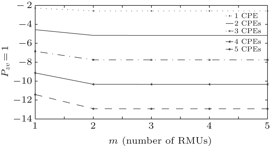	Fig.  5. Theoretical estimations of pzv versus the number of RMUs under the electromagnetic environment of 133.35-MHz frequency and 210-V/m field strength, with each of all the processing units having an upset probability of 0.0026.