


Start-up phase plasma discharge design of a tokamak via control parameterization method*
[Guo Shana) , Xu Kea) , Xu Chaob)†  , Ren Zhi-Gang
b) , Xiao Bing-Jiac) ]
, Ren Zhi-Gang|
|


†Corresponding author. E-mail: cxu@zju.edu.cn
*Project supported by the National Natural Science Foundation of China (Grant Nos. 61104048 and 61473253) and the National High Technology Research and Development Program of China (Grant No. 2012AA041701).
The tokamak start-up is a very important phase during the process to obtain a suitable equalizing plasma, and its governing model can be described as a set of nonlinear ordinary differential equations (ODEs). In this paper, we first estimate the parameters in the original model and set up an accurate model to express how the variables change during the start-up phase, especially how the plasma current changes with respect to time and the loop voltage. Then, we apply the control parameterization method to obtain an approximate optimal parameters selection problem for the loop voltage design to achieve a desired plasma current target. Computational optimal control techniques such as the variational method and the costate method are employed to solve the problem, respectively. Finally, numerical simulations are performed and the results obtained via different methods are compared. Our numerical parameterization method and optimization procedure turn out to be effective.
Nowadays, nuclear fusion has been regarded as the most promising resource because it is a clean energy resource which has tremendous potential.[1] The tokamak is believed to be the most promising fusion reactor. In a tokamak, the toroidal field is produced by electromagnets that surround the torus, and the poloidal field is generated by a toroidal electric current that is carried by the plasma. This current is induced inside the plasma with secondary electromagnet sets.[2] The structure of a tokamak is shown in Fig. 1.
 | Fig. 1. Schematic diagram of a tokamak chamber. |
Since the tokamak fusion reactor is a very complex device containing various connected subsystems with a large number of instabilities and during the working process it must deal with extremum temperature, high pressure, and great current, it has to face a lot of challenging control problems that urgently need to be solved. The control of the current profile in tokamak plasmas has been proved to be the enabler of advanced scenarios characterized by improved confinement, enhanced magnetohydrodynamic (MHD) stability, and possible steady-state operation.[3] There is a considerable interest in the start-up phase, as well as the tokamak breakdown process. This area is still far from completion.[4] In an operating fusion reactor, the electric field is applied to ionize the pre-fill gas and to ramp up the plasma current.[5] However, in the start-up of a reactor, either initially or after a temporary shutdown, the plasma will have to be heated to its operating temperature of greater than 10 keV. In designing the power supply system of a large tokamak, it is important to estimate the breakdown voltage and to decide the optimal voltage that we should supply to achieve successful start-up and a stable plasma current.[6] In this paper, we first study the properties of the zero-dimensional (0D) model, and in the future more complex models governed by partial differential equations (PDEs) can be used to generate more accurate results.
Now, we consider the most favourable situation that does not take into account impurities and escaping electrons. The model we use is described in Refs. [7]– [9], respectively. In this model, the term describing the average absorbed ECRH (electron cyclotron resonance heating) power is substituted into the energy balance equation for electrons. The energy balance equation for ions also takes into account the absorbed additional ICRH (ion cyclotron resonance heating) power. The energy balance equations for electrons and ions in the 0D approximation are written as the following ordinary differential equations:

The terms on the left-hand side denote the energy modification rates of electrons and ions. On the right-hand side, (3/2)(nekTe/τ E) and (3/2)(nikTi/τ E) are transport losses of energy and the other terms are the power inputs and power losses, whose specific meanings and expressions are listed in Table 1.
| Table 1. Notations in the system. |
The particle balance equations for electrons of concentration ne and neutrals of concentration n0 are governed by
Note that dne/dt and dn0/dt are the concentration modification rates of electrons and ions. n0neSi allows for neutral gas ionization and ne/τ p is the transport loss of particles.
The electric circuit equation for the plasma current Ip is governed by

which can be derived by Ohm’ s law directly. Lp = μ 0R(ln(8R/a)+ li/2 − 2) is the plasma column inductance and U is the loop voltage, which is considered as a control variable. Here, we set li ≈ 0.5 (flat current profile), and the other notations used in Eqs. (1)– (3) are listed in Table 1.
In the system of Eqs. (1)– (3), k, Ry, Wi, T0, li, μ 0 are physical constants and n, n0, Te, Ti, Ip are variables. In this paper, we will use the experimental parameters Vp, Vv, R, a, τ , Lp and the initial values of n, n0, Te, Ti, Ip which are parameters of the experimental advanced superconducting tokamak (EAST). EAST is the first shaped tokamak of mega-ampere scale to achieve plasma utilizing a fully superconducting poloidal field coil system located in Hefei, China.[10] Parameters of EAST that we have used are listed in Table 2.
| Table 2. EAST parameters. |
First of all, we rewrite Eqs. (1)– (3) as

where α = 2.2 × 10³ln Lp/(kVp), β = 0.16k− 1, γ = 1.6 × 10¹⁸Wi/1.5k, ξ = τ − 1, ζ = 1.6 × 10⁵k− 1,
and

where 
Because n0(n) = − (Vp/Vv)n + C, we then remove the equation for the ion concentration dn0, to obtain a new system including four equations and transform the system (1)– (3) to the following compact form:
For notational simplicity, we let X(t) = [n(t), Te(t), Ti(t), Ip(t)]T ∈ ℝ 4, then the system can be expressed as

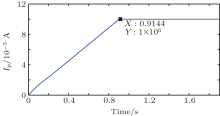
To figure out how the system works we first calculate values of the four variables for t ∈ [0, 2]. Figure 2 shows how the variables change when U = 6 V, PECRH = 4 MW, PICRH = 10 MW with initial values [nTeTiIp] = [2 × 10− 5 1 × 10− 3 3 × 10− 5 1]. It is obvious that in this situation Ip will increase rapidly and reach 1 × 10⁶ A at about 0.904 s. Now, we focus on determining the control of the loop voltage U to optimize other variables, particularly the plasma current Ip. In this paper, we only discuss a simple situation in which we separate the whole progress into two steps. The first step is to set U = 6 V which is actually the upper bound and PECRH = 4 MW, PICRH = 10 MW until Ip = 1 × 10⁶ A at the final time instant t = 0.904 s. The second step is to control U so that Ip can stay at 1 × 10⁶ A. Since the first step is stable, the main control purpose is to maintain the plasma current after t = 0.904 s. For convenience, we reset the initial time t = 0 s at the beginning of the second step, as well as initial condition
 | Fig. 2. Variable values in the first 2 s (U = 6 V). (a) n, (b) Te, (c) Ti, and (d) Ip. |

Thus, the altered problem is to minimize the following objective function:

The control U must satisfy 0 V ≤ U ≤ 6 V and 
Problem 1 Given the dynamic system (8) with initial condition (9), find an admissible control U ∈ [0 V, 6 V] such that the cost functional (10) is minimized.
To solve Problem 1, we will apply the control parametrization method introduced in Refs. [11]– [13]. Here we use two different methods.
Method 1 The control is approximated by a piecewise constant function with possible discontinuities at a set of fixed switching points.
The values of the piecewise constant functions then become decision variables to be selected optimally. In this paper, we will divide the time horizon [0, tf] into 10 subintervals [tk− 1, tk), k = 1, 2, 3, … , 10 and t0, t2, … , t10 is equally placed time points such that

and the control function U is approximated by a constant value on each subinterval denoted by σ k, then U can be expressed as

where χ [tk− 1, tk) : ℝ → ℝ is the indicator function defined by

and σ k satisfies 0 V ≤ σ k ≤ 6 V. For convenience, we use σ to denote [σ 1, σ 2, … , σ 10].
When we finish the control parameterization procedure, the dynamic system (8) becomes
and the cost functional (10) becomes
Now we can state the approximate parameter selection problem as follows.
Problem 2 Given the dynamic system (14) with initial condition (9), find admissible control parameter vector σ ∈ [0 V, 6 V] such that the cost functional (15) is minimized.
Method 2 The control is approximated by a polynomial U(t) = ξ 1t3+ ξ 2t2+ ξ 3t+ ξ 4, where ξ 1, ξ 2, ξ 3, ξ 4 ∈ ℝ , are the parameters to be optimized.
Now ξ 1, ξ 2, ξ 3, ξ 4 are decision variables to be selected optimally. The dynamic system (8) becomes
and the cost functional (10) becomes
When using Method 2, we must ensure that U(t) ∈ [0 V, 6 V]. Therefore, we add some inequality constraints generated by the sampling method. In this paper, we will divide the time horizon [0, tf] into 20 subintervals [tj− 1, tj), j = 1, 2, 3, … , 20 and t0, t2, … , t20 are equally placed time points. Then the inequality constraints can be described as 
Now, we can state the approximate parameter selection problem as follows.
Problem 3 Given the dynamic system (16) with initial condition (9), find admissible control parameters ξ 1, ξ 2, ξ 3, ξ 4 such that the cost functional (17) is minimized.
However, in some situation, it will be more convenient for the numerical computation if we transform the integral part of the cost functional to a terminal state of the dynamic system. Here, we define a new variable XJ satisfying

Notice that XJ(tf) equals cost functional J in Eq. (10), and we add XJ to the dynamic system (8). We introduce the following new state variable vector:
with the initial condition

Then, the cost functional (10) becomes

Now we can state the approximate parameter selection problem as follows.
Problem 4 Given the dynamic system (19) with initial condition (20), find admissible controls U ∈ [0 V, 6 V] such that the cost functional (21) is minimized.
Similarly we can apply Methods 1 and 2 to Problem 4 to obtain other approximate problems by changing the dynamic systems (14) and (16) into


Meanwhile, we change the cost functional Eqs. (15) and (17) into a terminal time representation


Problem 5 Given the dynamic system (22) with initial condition (20), find admissible control parameter vector σ ∈ [0 V, 6 V] such that the cost functional (24) is minimized.
Problem 6 Given the dynamic system (23) with initial condition (20), find admissible control parameters ξ 1, ξ 2, ξ 3, ξ 4 such that the cost functional (25) is minimized.
As problems 2, 3, 5, and 6 are optimal parameter selection problems in a canonical form then we can solve them as nonlinear optimization problems using the active-set[14] or SQP method.[15] Algorithm 1 below is the optimization algorithm for solving the approximate problem.
Algorithm 1
Step 1 Give an initial guess;
Step 2 Compute objective value and gradient value at the current points;
Step 3 If it is optimal, algorithm ends. Otherwise, go to Step 4;
Step 4 Calculate search direction;
Step 5 Determine optimal step length;
Step 6 Generate new parameter vector, then go back to Step 2.
There is a nonlinear optimization solver FMINCON in MATLAB which can automatically carry out Steps 3– 6. In spite of this, we need to supply the gradient formula of the cost functional. Here, we solve Problem 5 using the variational method.[16] We define the state variation with respect to σ as follows:

From Eq. (22), we have

Thus, we take the derivative with respect to σ to obtain
By differentiating with respect to time, we can obtain
Thus, Γ (· | σ ) is the solution of the following variational system:
with the initial condition

Now we can use the chain rule to compute the gradient of the cost functional with respect to the decision variables

By integrating with the nonlinear programming algorithm in MATLAB using this gradient, then Problem 5 can be solved numerically.
Next we introduce the costate method to compute the cost functional gradient. Here we compute Problems 2 and 3 using this method.
According to classical optimal control theory, [11] the Hamiltonian of Problem 2 can be defined by
where μ ∈ ℝ 4 is called the costate vector. Using the maximum principle, the costate system is defined by
Let μ (· | σ ) denote the solution of this costate system, then we can compute the cost functional gradient

We can use Simpson’ s rule to evaluate this integral term in Eq. (35). Let q be an even integer. Choose a partition 

then
The Hamiltonian corresponding to Problem 3 is defined as

and the rest of the computation is similar to Eqs. (34)– (36).
With the computation of gradient of the cost functional, Problems 2 and 3 can be solved numerically.
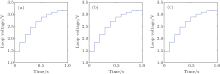
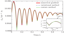
In simulation, we set the time interval [0, 1] and equally divide it into 10 subintervals. Then, we optimize the loop voltage U(l), l = 1, 2, … , 10. The numerical results of Method 1 are shown in Figs. 3 and 4. The curve of Ip during the whole start-up phase (both the first part in which U = 6 V and the second part in which optimal control is applied are included) is shown in Fig. 5. From these figures we can see that the optimal control is quite effective.
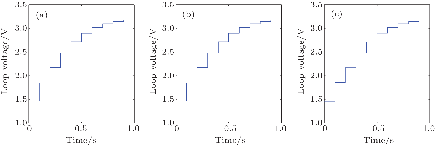 | Fig. 3. Optimization results of piecewise-constant loop voltage. (a) Optimation without gradient, (b) optimation with gradient in variational method, (c) optimation with gradient in costate method. |
 | Fig. 4. Optimization results of Ip with respect to piecewise-constant loop voltage. |
 | Fig. 5. Optimization results of Ip during the whole period. |
We can see the Ip curves fluctuate around the desired value (1 MA) and tend to be stable with the time increases. We set the same initial guess for the loop voltage parameters 
| Table 3. M1 computation time and optimized results. |
The advantage of M1 is that the loop voltage is piecewise-constant, which is easy to control. However, the smoothness of Ip cannot be ensured and the computation time is relatively long.
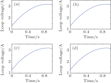
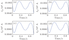
The loop voltage is in the parameterization form of 3-order polynomial about time t. Then, it can be expressed as U(t) = ξ 1t3+ ξ 2t2+ ξ 3t+ ξ 4, where ξ 1, ξ 2, ξ 3, and ξ 4 are optimal parameters. The numerical calculations of Method 2 are shown in Figs. 6 and 7. Table 4 illustrates the comparison of computing time and optimized results. The weight in the figures stands for the weight (λ ) of the control cost in the cost functional. It has influence on the optimal cost functional value, but has little impact on the optimal control parameters. Because there are only four parameters, the computing time is much less than that of Method 1 and the two methods (CM and VM) have some minor differences in values and time.
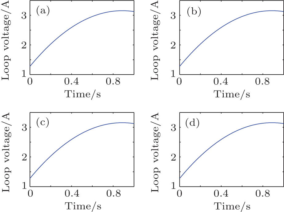 | Fig. 6. Optimization results of 3-order polynomial loop voltage. (a) VM with weight, = , 0, (b) VM with weight, = , 2000, (c) CM with weight, = , 0, (d) CM with weight, = , 2000. |
 | Fig. 7. Optimization results of Ip with respect to 3-order polynomial loop voltage. (a) Variational method with weight, = 0, (b) variational method with weight, = 2000, (c) costate method with weight, = 0, (d) costate method with weight, = 2000. |
| Table 4. M2 computing time and optimized results. |
Though the object value of M2 is slightly larger than M1, it is much faster.
We present an effective computational method for plasma current design during the start-up phase in a tokamak. The simulation results listed above have demonstrated that both of the control parametrization methods are effective. Besides, during the simulation progress, we have compared the variational method with the costate method to compute the cost functional gradient. It turns out that the costate method is much faster than the variational method while the final cost functional is quite similar, especially when we use Method 1, which spends longer time since it has more parameters to be decided and more numerical ODEs to be computed. Even though, there is still a great deal of room for improvement. For instance, in this paper we have designed the current curve during the whole time interval. However, in many situations, we only care about the states of the terminal time and do not need to track a fixed current curve. In our future work, we will consider another situation in which we only set the terminal state constraints and it will generate the optimal current curve automatically without any additional constraints.
Remark 1 While using the variational method, it may need to compute the dynamic system and the variational system separately. This means that we need to compute the dynamic system first and then use the interpolation of the variable values to compute the variational system, because the ODEs may be singular and give wrong results if we put them together.
Remark 2 When it comes to the costate method, XJ(t) is not suitable to be added, because we will encounter a problem when computing ∂ H/∂ XJ.
| 1 |
|
| 2 |
|
| 3 |
|
| 4 |
|
| 5 |
|
| 6 |
|
| 7 |
|
| 8 |
|
| 9 |
|
| 10 |
|
| 11 |
|
| 12 |
|
| 13 |
|
| 14 |
|
| 15 |
|
| 16 |
|