

Theoretical analysis of transcranial Hall-effect stimulation based on passive cable model
[Yuan Yi†a)  , Li Xiao-Li‡
b), c) ]
, Li Xiao-Li‡]
|
|


†Corresponding author. E-mail: yuanyi513@ysu.edu.cn
‡Corresponding author. E-mail: xiaoli@bnu.edu.cn
*Project supported by the National Natural Science Foundation of China (Grant Nos. 61273063 and 61503321), the China Postdoctoral Science Foundation (Grant No. 2013M540215), the Natural Science Foundation of Hebei Province, China (Grant No. F2014203161), and the Youth Research Program of Yanshan University, China (Grant No. 02000134).
Transcranial Hall-effect stimulation (THS) is a new stimulation method in which an ultrasonic wave in a static magnetic field generates an electric field in an area of interest such as in the brain to modulate neuronal activities. However, the biophysical basis of simulating the neurons remains unknown. To address this problem, we perform a theoretical analysis based on a passive cable model to investigate the THS mechanism of neurons. Nerve tissues are conductive; an ultrasonic wave can move ions embedded in the tissue in a static magnetic field to generate an electric field (due to Lorentz force). In this study, a simulation model for an ultrasonically induced electric field in a static magnetic field is derived. Then, based on the passive cable model, the analytical solution for the voltage distribution in a nerve tissue is determined. The simulation results showthat THS can generate a voltage to stimulate neurons. Because the THS method possesses a higher spatial resolution and a deeper penetration depth, it shows promise as a tool for treating or rehabilitating neuropsychiatric disorders.
Transcranial magnetic stimulation (TMS) is a noninvasive brain stimulation method that rapidly changes the magnetic field to induce a weak electric current. TMS can cause the neurons of the brain to depolarize or hyperpolarize. TMS has been widely tested as a tool for treating and rehabilitating various neurological and psychiatric disorders, including Parkinson’ s disease, Alzheimer’ s disease, autism, depression, epilepsy and stroke.[1– 5]
However, the spatial resolution of TMS is larger than several centimeters because the magnetic field cannot be effectively concentrated.[6] Additionally, the stimulation distance of the TMS is limited because the alternating magnetic fields obey Laplace’ s equation.[7] To address this problem, an H-coil was developed to improve the stimulation distance of the TMS.[8, 9] However, deep TMS still cannot stimulate deep brain areas.
In comparison with TMS, transcranial ultrasound stimulation (TUS), a new noninvasive brain stimulation method, can perform a deep stimulation with spatial resolutions of approximately 2 mm.[10– 14] The effectiveness of TUS has been demonstrated in animals and humans.[15– 17] Through low-intensity ultrasound, TUS can modulate voltage-gated Na+ and Ca2+ channel activity to evoke the action potentials of neurons; [18] however, the mechanisms of TUS remain to be elucidated.
In this paper, we study transcranial Hall-effect stimulation (THS) that integrates the advantages of TMS with those of TUS. THS can generate an electric field in a static magnetic field by using ultrasonic waves to stimulate the brain tissues. The ultrasonic waves are generated by the focused ultrasound transducer and the static magnetic field came from the permanent magnet or power coil placed in both sides of the sample.[19, 20] The principles behind THS are based on the Hall-effect, which describes the charge separation in a conductor moving in a magnetic field.[21– 24] The spatial resolution of THS is determined by the size of the ultrasonic spot; therefore, it has the same spatial resolution as the TUS. At the same time, the ultrasound stimulation has a good penetration depth and the magnetic field strength is not the largest in the surface and monotonically decreases over the stimulation distance. Therefore, THS possesses a greater spatial resolution and a higher penetration for brain stimulation. Here, we use theoretical derivation and numerical simulation methods to study the mechanism of THS for modulating neural activities.
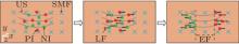
The schematic of an ultrasonically induced electric field in a static magnetic field on a nerve is shown in Fig. 1. The action of a focused ultrasonic wave moves charged ions along the y-axis direction in the nerve tissue. Because a static magnetic field is perpendicular to the movement direction of the charged ions, the Lorentz force action on the ions can be induced in the nerve tissue. The Lorentz force separates the positive ions from negative ions in opposite directions, thereby forming an electric field. In this study, we intend to estimate the voltage distribution in the nerve tissue generated by an ultrasonically induced electric field.
 | Fig. 1. Schematic diagram of ultrasonically-induced electric field in a static magnetic field (SMF) in a nerve fiber. (Left) The action of focused ultrasonic wave oscillates charged ions along the y axis. A static magnetic field is perpendicular to the movement direction of the charged ions. (Middle) Lorentz force generated on ions due to the interaction of the ultrasound and magnetic fields. (Right) The Lorentz force moves the positive and negative ions in opposite directions and subsequently, forms an electric field between the ions. US: ultrasound, SMF: static magnetic field, PI: positive ion, NI: negative ion, LF: Lorentz force, EF: electric field. |
Assuming that an ion in a conductive medium has a charge q, and that the ultrasonic wave of an electric field oscillates the ion with a velocity υ along the ultrasound penetration direction in the medium, in a constant static magnetic field B0, a Lorentz force F can then be expressed by

The ion velocity υ generated by the ultrasonic wave is a key parameter in the above equation. The magnitude of ion velocity v is related to the sound pressure p by

where ρ is the tissue density and c0 is the ultrasound speed.
When the pressure wave, the static magnetic field and the ion velocity are perpendicular to each other, namely υ = vz and B0 = B0y, the Lorentz force F can be expressed as

Combining Eqs. (2) and (3), according tox = z × y, we obtain the following equation:

As is well known, the relationship between the electric field E and the Lorentz force F obeys the following classical relation equation:

Combining Eqs. (4) and (5), we obtain the following equation:

The focused ultrasound is an ultrasound beam propagating in the z direction and has a three-dimensional distribution in space. There is an ultrasound beam that has axial symmetry with a radial profile given by p(r, t) in the x– y plane, where

The nerve fiber is along the x-axis direction. Since there is no effect of the distribution of ultrasound intensity along the y- and z-axis directions on the nerve, we only consider the distribution of ultrasound intensity along the x-axis direction shown in Eq. (7)

where p0 is the maximum intensity of the sound pressure, I(t) is the time step function.
Combining Eqs. (6) and (7), the electric field E (x, t) generated by an ultrasound can be written as

As the excitation source of ultrasonic-magnetic stimulation, E (x, t) is used for modulating neural activities.
To calculate the voltage distribution in the nerve tissue that is ultrasonically generated by the static magnetic field, a passive cable model is employed[25] as shown in Fig. 2. In the passive cable model, there are three underlying assumptions: (i) the intracellular potential is only a function of the axial distance x along the length of the fiber; (ii) the axoplasm behaves like a linear, and for Ohmic conductor its resistance per unit length is ri; (iii) the extracellular potential produced by the fiber’ s own activity is negligible.[25, 26]
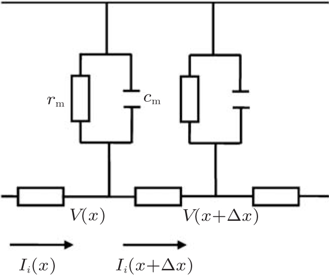 | Fig. 2. Electrical circuit of the passive cable model. The intracellular space is represented by a resistance per unit length ri, the membrane by a resistance times unit length rm and by a capacitance per unit length cm. The extracellular potential is assumed to be zero. |
For a cylindrical conductor of infinite length, the cable equation with no myelinated nerve fibers according to Kirchhoff’ s law circuit[25] is

where

is a length constant, τ = cmrm is a time constant, rm is the resistance times a unit length, cm is the capacitance per unit length, and ri is the membrane resistance per unit length.
In the passive cable model, when the nerve fiber is influenced by an electric field E(x, t) parallel to the nerve fiber, equation (9) can be written as[25]

Equation (10) is a cable model for electric field stimulation. We can obtain the analytical solutions of the voltage distribution by solving Eq. (10) for V(x, t).
To simplify the calculation, we assume that

Then, equation (10) can be expressed as

Using Fourier transforms as shown in the appendix, we solve Eq. (12) for V(x, t):
where c2 = λ 2/τ and b = 1/τ .
According to Eq. (8), g(ζ , t − η ) can be expressed as

Combining Eqs. (13) and (14), we obtain the analytical solution for the voltage distribution as follows:
Equation (15) can be used to estimate the electric field produced by ultrasound in the static magnetic field.
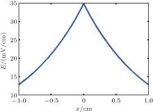
To simulate the distribution of an electric field, we assume that the intensities of the magnetic field and the ultrasound are 3 T and 5 MPa, respectively. According to Eq. (8) and the simulation results, the electric field E(x, t) along the x axis is shown in Fig. 3. The intensity of the electric field decreases with increasing spatial distance.
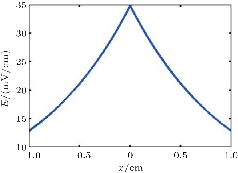 | Fig. 3. Distribution of electric field E(x, t) along the x axis. |
To simulate the voltage distribution induced by the electric field, we set the parameter values of a few physical variables, which are given in Table 1.[25] In the passive cable model, the intracellular space is modeled by a resistance per unit length ri = Ri/π r2, where Ri is the resistivity of the axoplasm and r is the radius of the fiber. The resistance per membrane length unit of the membrane is rm = Rm/2π r, where Rm is the resistivity of the membrane. The membrane capacitance per unit length is cm = Cm2π r, where Cm is the membrane capacitance per unit area.
| Table 1. Parameters of physical variables and nerve. |
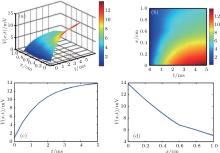
To evaluate the voltage distribution in the nerve that is ultrasonically induced by the presence of a static magnetic field, we first analyze the effects of the stimulation time and the distance on voltage distribution. The parameters of the passive cable model are listed in Table 1, and the intensities of the magnetic field and ultrasound are 3 T and 5 MPa, respectively. Based on Eq. (15), the simulation results are shown in Fig. 4. Figure 4(a) shows the three-dimensional voltage distribution over the stimulation time and the distance from the center of the ultrasonic source. Figure 4(b) shows the two-dimensional voltage distribution corresponding to the data presented in Fig. 4(a). The simulation results indicate that the intensity of the voltage distribution is influenced by two parameters: the stimulation time and the distance from the center of the ultrasonic source. As shown in Fig. 4(c), when the stimulation time is constant, the intensity of the voltage distribution is strongest in the center of the ultrasound-focused source, and it gradually decreases with increasing distance from the center. As shown in Fig. 4(d), when the distance from the center of the ultrasonic source is constant, the intensity of the voltage distribution gradually increases with increasing stimulation time.
 | Fig. 4. (a) Three-dimensional voltage distribution against the stimulation time and the distance from the center of the ultrasonic spot. (b) Two-dimensional voltage distribution corresponding to panel (a). (c) The simulation results at a constant stimulation time of 5 ms. (d) The simulation results at a constant distance from the center of the ultrasonic spot. |
Now we analyze the effects of the intensity of the magnetic field and the amplitude of the sound pressure on voltage distribution. The parameters’ values of the passive cable model are listed in Table 1. The intensity of the magnetic field ranges from 0 T to 7 T and the amplitude of sound pressure is in a range from 0 MPa to 2 MPa. Figure 5(a) shows the three-dimensional voltage distribution versus the intensity of the magnetic field and the sound pressure. Figure 5(b) shows the two-dimensional voltage distribution corresponding to the data presented in Fig. 5(a). The intensity of the voltage distribution increases with increasing intensities of the magnetic field and the sound pressure amplitude. When the intensity of magnetic field is constant, the intensity of the voltage distribution linearly increases with increasing sound pressure amplitude (Fig. 5(c)). The intensity of the voltage at an ultrasound pressure of 14 MPa increases as the intensity of the magnetic field increases (Fig. 5(d)).
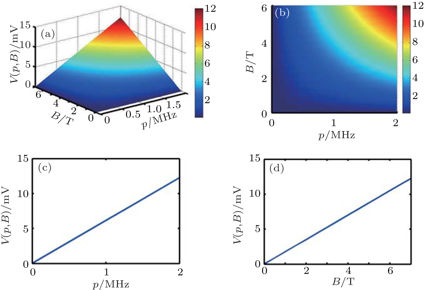 | Fig. 5. (a) Three-dimensional voltage distribution versus the intensity of magnetic field and sound pressure amplitude. (b) Two-dimensional voltage distribution corresponding to panel (a). (c) The simulation results at a constant magnetic field. (d) The simulation results at a constant sound pressure amplitude. |
In this study, we propose and calculate an ultrasonically induced voltage distribution in a nerve tissue based on a passive cable model. The proposed method can be used to calculate strength duration curves for various pulse shapes.[26] For the passive cable model, the calculation results show that the voltage distribution is a function of the sound pressure amplitude, intensity of the magnetic field, stimulation time and distance from the center of the ultrasonic source. The simulation results show that the voltage intensity increases with sound pressure amplitude, intensity of the magnetic field and stimulation time but decreases as the distance from the center of the ultrasonic source increases. Therefore, to enhance the voltage intensity in deep brain tissue, we can apply a highly focused ultrasound transducer on a single spot, at strong sound pressure and for a long stimulation time. However, the sound pressure amplitude would be limited to avoid damaging surrounding tissues; the recommended maximum limit for diagnostic imaging applications is 190 W/cm2.[27] The intensity and the sound pressure amplitude are related by the formula 
The spatial resolution and the penetration depth of THS are determined by the size of the ultrasound; therefore, THS has the same spatial resolution and penetration depth as the ultrasound stimulation. The basic mechanisms of THS and ultrasound stimulation are different from each other. The basic mechanism of THS is that the electric field is generated by the underlying static magnetic field and ultrasonic waves in nerve tissues. The basic mechanism of ultrasound stimulation is still unclear until now, and the possible mechanism of ultrasound stimulation is that ultrasound produces effects on viscoelastic neurons and their surrounding fluid environments, thus changing the membrane conductance.
Passive cable model that can also predict the transmembrane responses was used to evaluate the stimulation of the nerve fiber by electrical stimulation or magnetic stimulation in previous studies.[25, 26, 29, 30] In our study, the passive cable model is used to investigate the mechanism of THS of neurons. The stimulus source of THS, which is the electric field induced by ultrasound and magnetic field, is similar to electrical stimulation and magnetic stimulation. Therefore, the passive cable model is suitable to explaining the mechanism of THS of neurons.
In previous studies, Norton established the Maxwell equation combining the ultrasound and magnetic field and obtained the distribution of electric field from the macroscopic aspect.[7] In our study, we obtain the analytical solution for the voltage distribution based on the passive cable model of intracellular potential from the microcosmic aspect. Therefore, the model for the electric field in our paper differs from that presented in Norton’ s paper. Campanella[31] investigated the sound waves generated by the Hall effect with electric field and magnetic field in electrolytes. It is the inverse process of THS that the electric field was generated by the Hall effect with sound waves and magnetic field in electrolytes.
Ultrasonically induced electric fields in the presence of magnetic fields have been successfully demonstrated and can be used as a novel imaging method, i.e., Hall effect imaging.[32, 33] Hall effect imaging can be used for imaging nerve tissues. In this study, we investigate ultrasonically induced voltages in nerve tissues to stimulate neurons. The herein described method can be used for simultaneously stimulating and imaging nerve tissues. This can provide real-time monitoring during neuromodulation procedures.
In this study, on the basis of a passive cable model, we calculate the voltage distribution in a nerve induced by ultrasound wave in the presence of a magnetic field. The simulation results of the voltage distribution in the nerve indicate that this method can be used to generate sufficient voltage to stimulate neurons. Thus, it has the potential for treating and rehabilitating neuropsychiatric disorders, such as Alzheimer’ s disease, autism and Parkinson’ s disease.
Here we solve Eq. (12) with Fourier transform.
Assuming that c2 = λ 2/τ and b = 1/τ , equation (12) can be expressed as

Apply Fourier transform to x, then we will obtain

where V (w, t) and g (w, t) are the image functions of V (x, t) and g (x, t), respectively.
Consolidating Eq. (A2), we obtain

Both sides of Eq. (A3) are multiplied by e(w2c2+ b)t, then equation (A3) can be expressed as
Equation (A4) can be expressed as

When t = 0, the voltage distribution V = 0 and

Combining Eqs. (A5) and (A6), we obtain

Equation (A7) can be expressed as

Use the inverse Fourier transform to Eq. (A8), then we will obtain
As is well known,

According to Eqs. (A9) and (A10), we obtain
Using the coordinate transformationτ = t − η , we obtain
| 1 |
|
| 2 |
|
| 3 |
|
| 4 |
|
| 5 |
|
| 6 |
|
| 7 |
|
| 8 |
|
| 9 |
|
| 10 |
|
| 11 |
|
| 12 |
|
| 13 |
|
| 14 |
|
| 15 |
|
| 16 |
|
| 17 |
|
| 18 |
|
| 19 |
|
| 20 |
|
| 21 |
|
| 22 |
|
| 23 |
|
| 24 |
|
| 25 |
|
| 26 |
|
| 27 |
|
| 28 |
|
| 29 |
|
| 30 |
|
| 31 |
|
| 32 |
|
| 33 |
|