It is well known that the cubic–quintic nonlinear Schrödinger equation (NSE)

Recently, the symplectic method was developed to solve the Hamiltonian system, and it is superior to the nonsymplectic ones, especially for many-step and long-time computation.^[11–13] Up to now, it has been applied to many fields, such as the quantum mechanics,^[14] molecular dynamics,^[15] Bose–Einstein condensates,^[16–20] solar system dynamics, and general relativity.^[21–25] A fourth-order, three-stage, symplectic integrator with small numerical error has been used, and a method of fast Lyapunov indicator has been applied in studying the dynamics of the system.^[21,23] The Lyapunov exponents and the fast Lyapunov indicators are chaotic indicators independent of the dimensionality of phase space, and they are widely used in higher-dimensional systems to distinguish chaos from order.^[24] For example, the fast Lyapunov indicator has been used in the three-body problem and compact binary systems to identify chaos.^[26–28] High-order symplectic finite difference time-domain schemes have been used in the Maxwell’s equations^[29] as well as in the Schrödinger equation,^[30,31] and good numerical results have been reported. As for the nonlinear Schrödinger equation, a symplectic finite-dimensional reduction approach is used, which is proved to be effective.^[32] The cubic NSE has a symplectic structure and thus can be solved by the symplectic method. In Ref. [33], we have discussed the dynamic behaviors of the cubic NSE by the symplectic scheme. Since the cubic–quintic NSE can be transformed into a Hamiltonian system, it can also be solved by the symplectic algorithm.

In this paper, the dynamics of the cubic–quintic NSE are studied by the symplectic method and we concentrate on the impact of the quintic term. We observe that the system will exhibit interesting behaviors, and the changing process of the phase trajectories is various for different cubic nonlinear parameter q with the increase of the quintic nonlinear parameter g. The study on the contributions from the fifth degree terms may be important for some future modellings, and this topic is related to a rather broad area of mathematical physics.

In Section 2, the symplectic method is extended into the cubic–quintic NSE. In Section 3, the conservation of the conserved quantities is discussed. In Section 4, the basic dynamic properties of the NSE with different cubic nonlinear parameter q and increasing quintic nonlinear parameter g are illustrated. Conclusions are given in Section 5.

Consider the cubic–quintic NSE (1) with the following periodic boundary condition:

Therefore the cubic–quintic NSE (1) can be rewritten in the Hamiltonian formalism which has the symplectic structure, and its time evolution in phase space is symplectic transformation. A symplectic method is a method that can preserve the symplectic structure of the Hamiltonian system, and it is a reliable method to solve this kind of problem. For example, the second order symplectic scheme is^[11,34]

In the above, we write the NSE (1) into the Hamilton canonical equation (3), which is of infinite-dimension and has the symplectic structure. Then we discretize equation (3) by the symplectic method and obtain equation (5), which is finite dimensional. The truncation approximations are asymptotic in nature. The schemes we considered here are implicit, and convergence can be achieved by iterations. The finite-dimensional Hamiltonian canonical equation (5) reserves the symplectic structure and the property of norm conservation of the original system (3), then it is natural to use the symplectic method which can preserve the symplectic structure of the discrete Hamiltonian canonical equation (5) as well as the discretized norm of the wavefunction.

In computing the NSE, Runge–Kutta methods are also commonly used and they have been generalized to any given order by Butcher to prevent the error accumulation. The multisymplectic method can also be applied in the Hamiltonian system. For example, Hong et al. presented a conservation law which is essential and intrinsic for a class of varying coefficient NSE.^[36] The mid-point scheme is a basic algorithm and can be used directly to the NLE, which is adopted in this paper.

It is easy to show that the cubic–quintic NSE (1) has conserved quantities,^[1] for example, the quasiparticle number

In numerical simulations, we choose the initial condition as

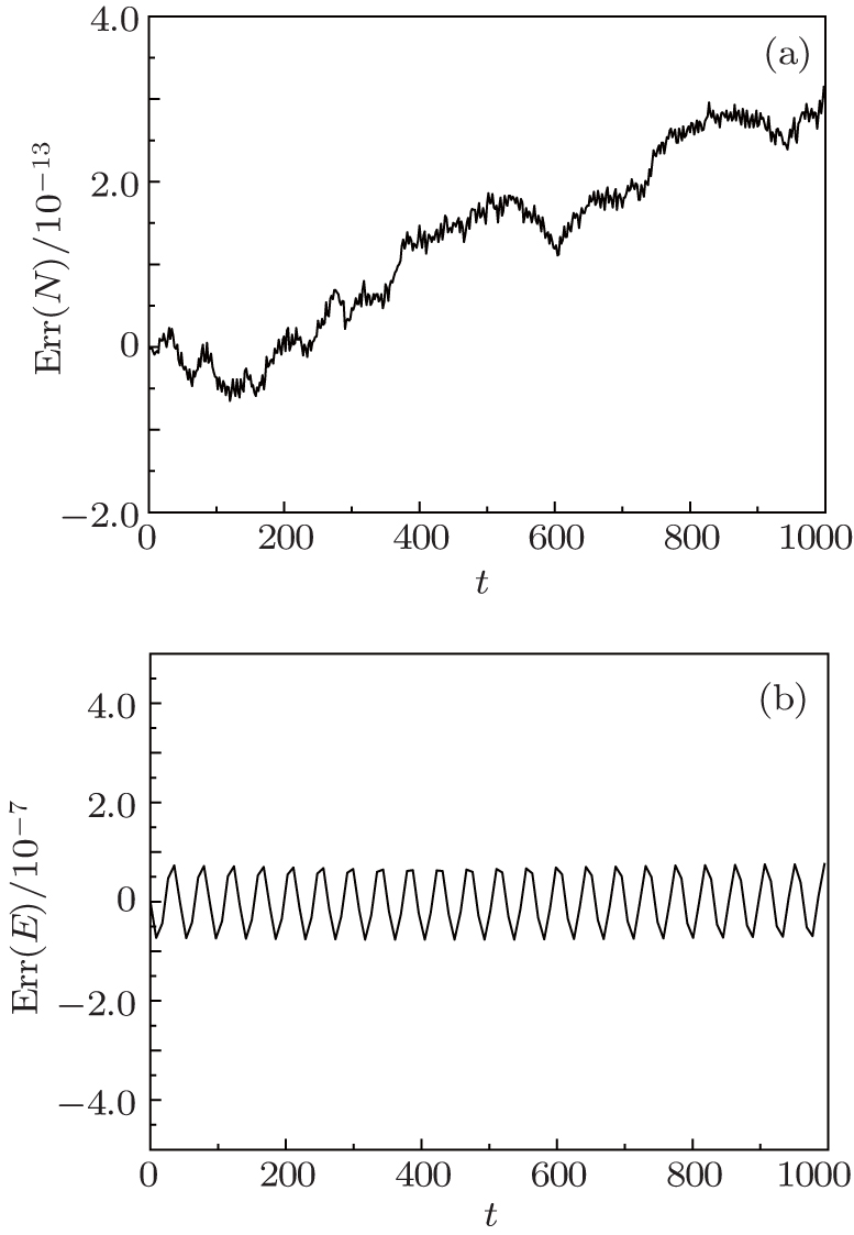
The numerical solution of Eq. (1) is obtained by the mid-point scheme (9) with the second-order central space difference (4). The mid-point scheme is implicit, an appropriate temporal step size τ should be chosen and convergence can be achieved through simple iterations.^[37] In computation, we choose the space step h = L/64 and time step τ = 0.001. The Seidel iteration method is adopted. The computation time is from t = 0 to t = 10³ and the total computation step is 10⁶. The results of the conserved quantities with q = 0.001 and g = 0.001 are shown in Fig. 1, where Err(N) and Err(E) are the errors of the quasiparticle number and the total energy, respectively. From Fig. 1, we can see that the quasiparticle number is preserved to 10⁻¹³ and the total energy to 10⁻⁸ for long time computation. We also find that the error of the total energy oscillates periodically near the zero point during the long time evolution. It is assured that our method preserves these quantities well and thus is reliable.

Fig. 1.

	Figure Option ViewDownloadNew Window
	Fig. 1. Conserved quantities of the cubic–quintic NSE with q = 0.001 and g = 0.001. Evolution of the errors of (a) the quasiparticle number and (b) the total energy.

To analyze the dynamic properties of the cubic–quintic NSE (1) in long time evolution, we use the phase space (A, A_t) at x = L/2 defined as

Here, the amplitude is taken as A(L/2,t) = ∣E(L/2, t)∣ − 1, the original wave oscillating around value 1 is modulated to oscillate around value 0. Moon^[7] experimentally guessed that the origin (A,A_t) = (0,0) could be a saddle for q = 1 and g = 0, and observed that a homoclinic orbit (HMO) would appear when θ is slightly larger than 45°. In our study, we consider the case of θ = 45.18° and study the dynamics of equation (1) with different cubic and quintic parameters under the initial condition (15), where q is in the range of 0.01–1.0115 and g is in the range of 0–0.25. Since the result of long time evolution is almost the same for t > 10³, we only discuss the dynamic properties for 0 ≤ t ≤ 10³.

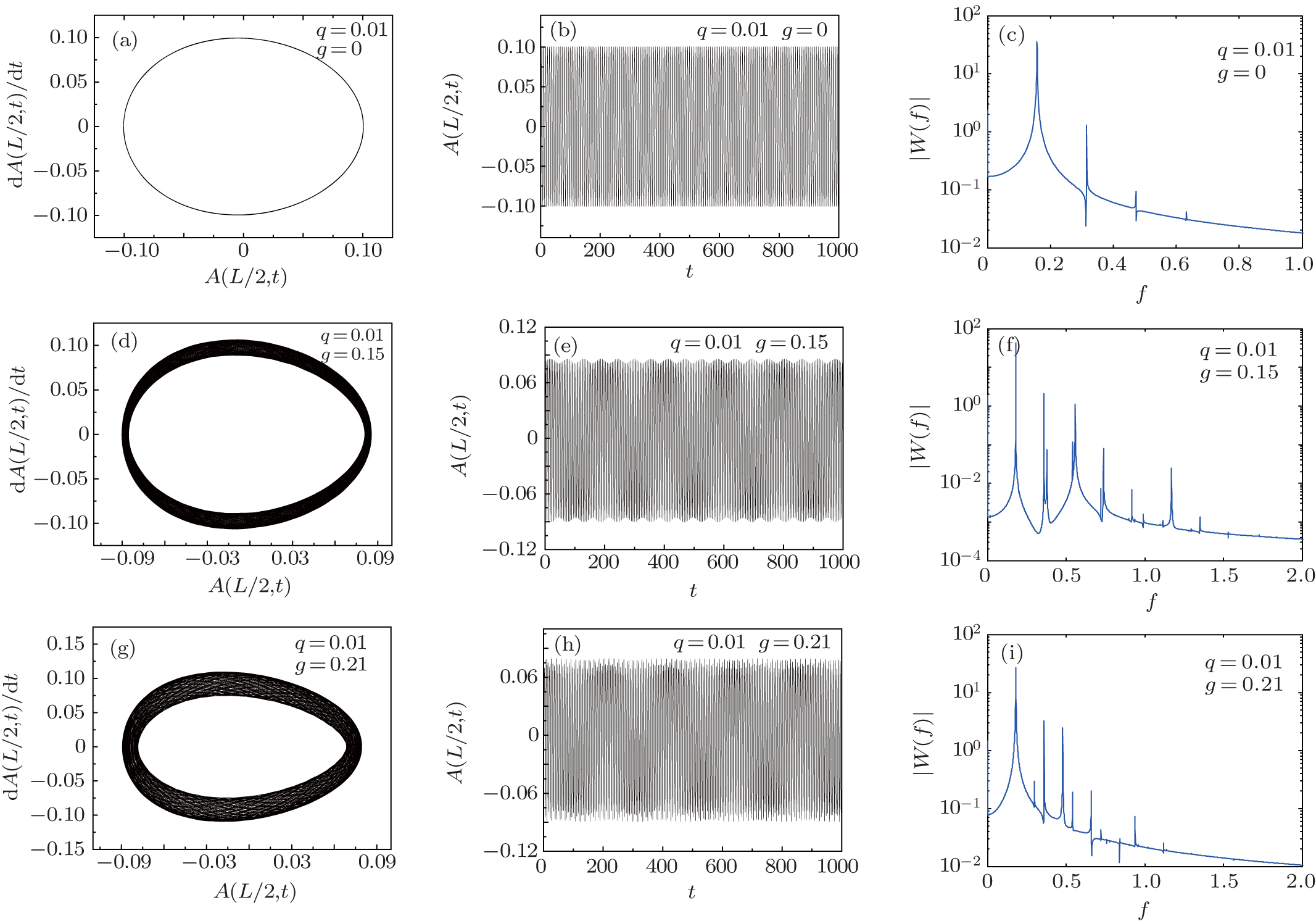
Figure 2 shows the numerical results with θ = 45.18°, q = 0.01, and different quintic parameter g. Figures 2(a), 2(d), and 2(g) are phase trajectories in the phase space (A,A_t). Figures 2(b), 2(e), and 2(h) are the time evolutions of the amplitude of the wave, A(L/2, t). Figures 2(c), 2(f), and 2(i) are the corresponding Fourier spectra of A(L/2, t). For q = 0.01 and g = 0, the phase trajectory is a single loop, as shown in Fig. 2(a), it is an elliptic orbit and the origin (A,A_t) = (0,0) is an elliptic point. The time series of A(L/2, t) is exact recurrent motion as shown in Fig. 2(b), and the spectrum is discrete with peaks of equal intervals as shown in Fig. 2(c). We can see that the system has a periodic solution and the trajectory in phase space is a periodic recurrent orbit with a coherent structure. For q = 0.01 and g = 0.15, the trajectory in the phase space becomes more thicker and no longer exactly periodic as shown in Fig. 2(d). The time series of A(L/2, t) is quasirecurrent motion as shown in Fig. 2(e), and the spectrum of the trajectory is a discrete distribution with some subharmonics as shown in Fig. 2(f). We can see that the system has a quasirecurrent solution when we add a small quintic nonlinearity g. For q = 0.01 and g = 0.21, the trajectory in phase space becomes thicker, which indicates a quasirecurrent solution. The time series of A(L/2, t) is not an exact periodical temporal evolution and the spectrum of the trajectory is a discrete distribution with more subharmonics. It shows that the system has a quasirecurrent solution when the nonlinearity g is increased. From Fig. 2, we can see that there exists an exact periodic recurrence solution for a small cubic parameter, and it becomes quasirecurrence with the increase of the quintic parameter.

Fig. 2.

	Figure Option ViewDownloadNew Window
	Fig. 2. Numerical solutions of the cubic–quintic NSE by symplectic method with θ = 45.18°, q = 0.01, and different parameter g. Panels (a), (d), and (g) are the phase trajectories; panels (b), (e), and (h) are the time evolutions of A(L/2, t); and panels (c), (f), and (i) are the Fourier spectra of A(L/2, t) corresponding to panels (b), (e), and (h), respectively.

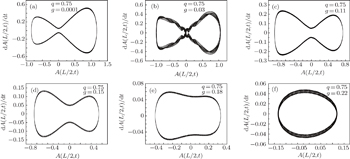
For Eq. (1) with weak cubic nonlinearity, the trajectory in phase space is an elliptic orbit and the origin (A,A_t) = (0,0) is an elliptic point. With the increase of the cubic parameter q (q > 0.5), the periodic orbit will shrink to the origin (A,A_t) = (0,0) along the A(L/2, t) = 0 axis, and become two loops. Simultaneously, the origin becomes a saddle and the trajectory in phase space is a homoclinic orbit (HMO).^[33] Numerical results with q = 0.75 and increasing quintic parameter g are shown in Fig. 3. Figure 3(a) gives a typical HMO with q = 0.75 and g = 0.0001. Figure 3(b) shows a thicker phase trajectory with q = 0.75 and g = 0.03. This trajectory is still a HMO but is a quasirecurrent solution of many-cycle. When g is increased to 0.11 and 0.15, the trajectories are again the regular HMO as shown in Figs. 3(c) and 3(d). If g increases further, the HMO will deviate from the origin (A,A_t) = (0,0) along the A(L/2, t) = 0 axis, and become one loop. Simultaneously, the origin becomes an elliptic point and the trajectory becomes an elliptic orbit as shown in Figs. 3(e) and 3(f), which indicates the quasirecurrent solution of the system. From Fig. 3, we can see that when q = 0.75, the phase trajectory will change from HMO to elliptic orbit with the increase of the quintic parameter.

Fig. 3.

	Figure Option ViewDownloadNew Window
	Fig. 3. Phase trajectories of the cubic–quintic NSE by symplectic method with θ = 45.18°, q = 0.75, and different parameter g: (a) g = 0.0001, (b) g = 0.03, (c) g = 0.11, (d) g = 0.15, (e) g = 0.18, (f) g = 0.22.

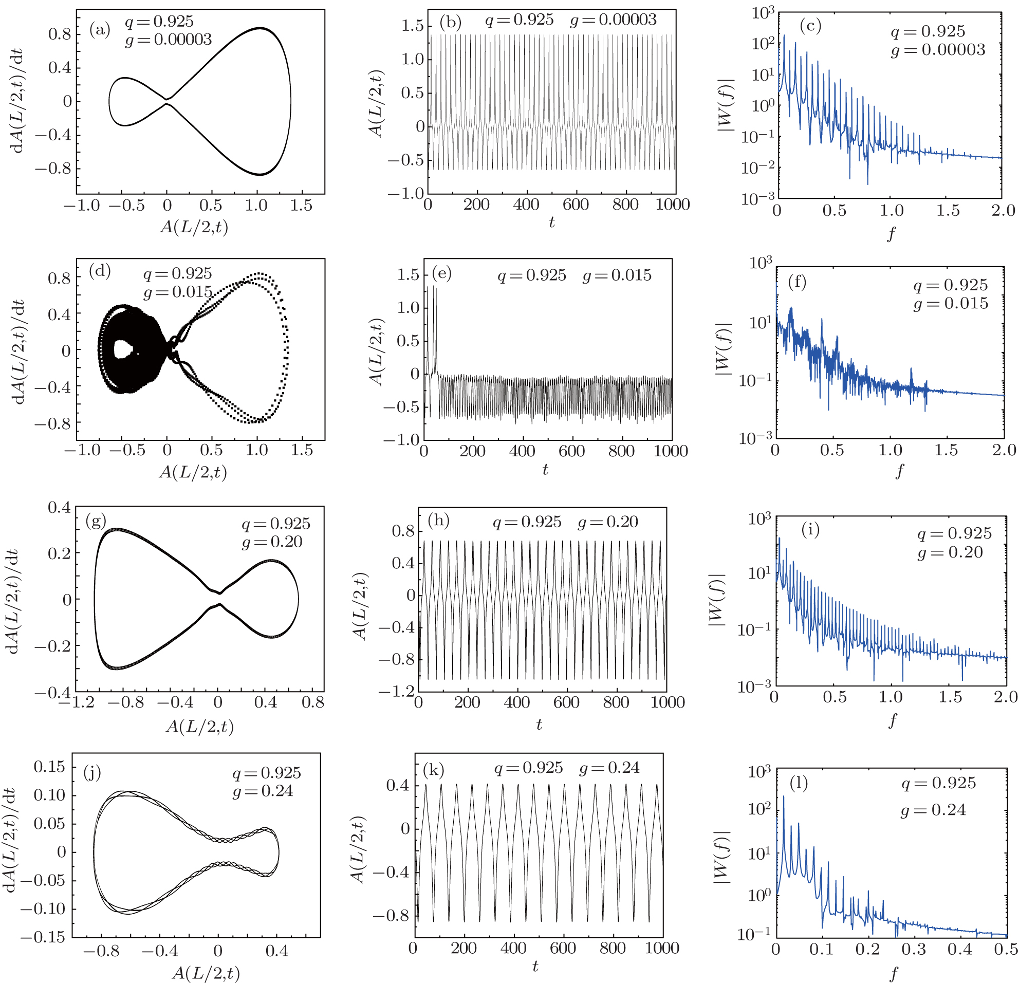
When q is increased, we observe more complex phenomena. Numerical solutions with q = 0.925 and different g are shown in Fig. 4. Figure 4(a) shows a typical regular HMO with q = 0.925 and g = 0.00003, and the left loop is smaller than the right one. The time series of A(L/2, t) is periodic and the spectrum is discrete. It is periodic recurrent motion. When g is increased to g = 0.015, the periodic orbit is broken and the irregular HMO crossings appear as can be seen in Fig. 4(d). The temporal evolution of A(L/2, t) shows the typical chaotic character, and the Fourier spectrum is noise-like and has a broadband structure, which indicates the irregular motion of the system. Therefore a larger quintic nonlinear parameter g may lead to irregular HMO crossings, and the system will exhibit a stochastic behavior. With the increase of g, the recurrent solution is again observed at g = 0.20 as shown in Figs. 4(g)–4(i). It is a regular HMO, but the left loop is bigger than the right one, which is opposite to that in Fig. 4(a). For g = 0.24, figure 4(j) shows an interesting phenomenon, a recurrent solution of three-cycle, and the three cycles are intertwisted together and form a HMO. From Fig. 4, we conclude that for q = 0.925 and increasing g, the system changes as follows: the periodic recurrent motion → the stochastic motion or irregular motion → the regular HMO → the HMO of recurrent motion of three-cycle.

Fig. 4.

	Figure Option ViewDownloadNew Window
	Fig. 4. Numerical solutions of the cubic–quintic NSE by symplectic method with θ = 45.18°, q = 0.925, and different parameter g. Panels (a), (d), (g), and (j) are the phase trajectories, panels (b), (e), (h), and (k) are the time evolutions of A(L/2, t), and panels (c), (f), (i), and (l) are the corresponding Fourier spectra.

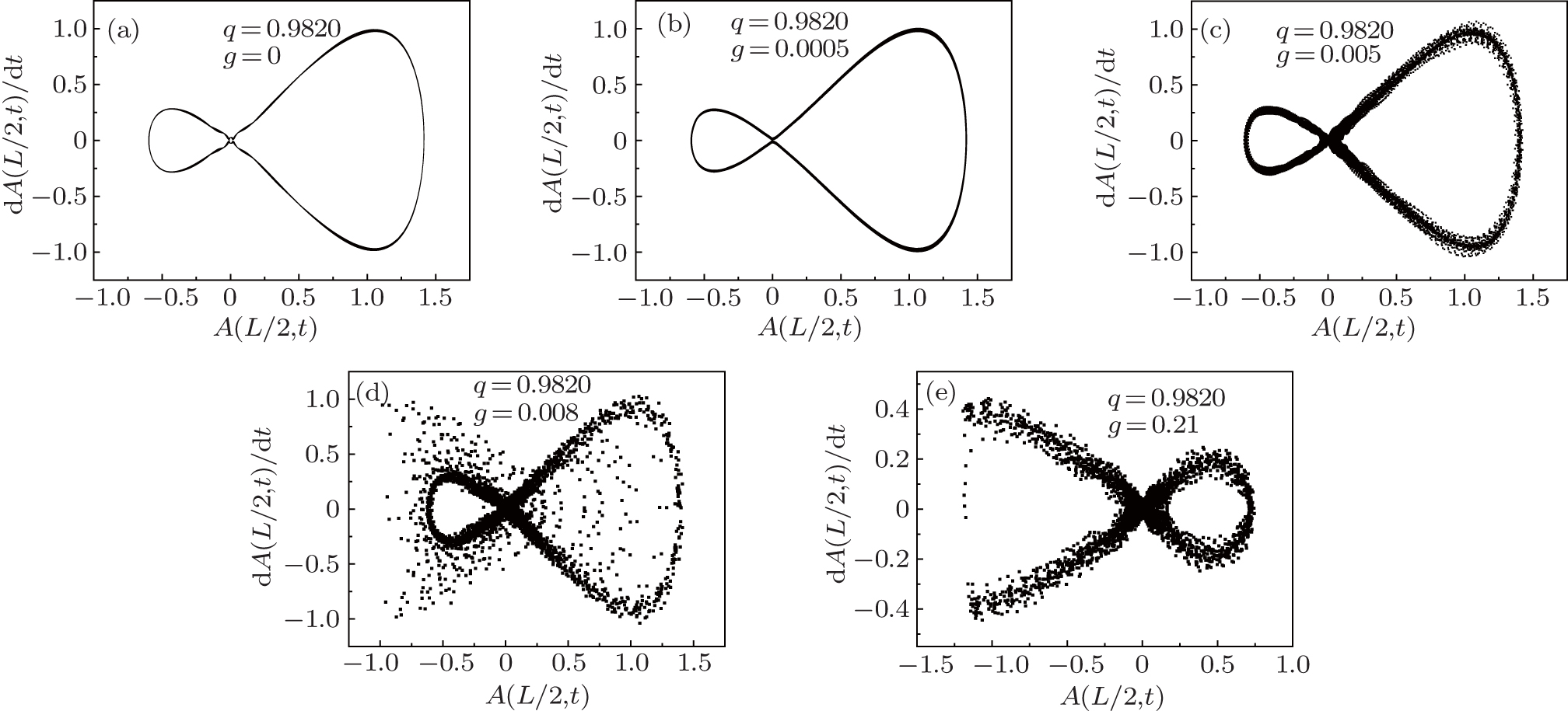
Figure 5 gives the phase trajectories for q = 0.9820 and different parameter g. Figure 5(a) shows the result of g = 0, the phase trajectory presents recurrent motion and is a HMO. Figure 5(b) shows the result of g = 0.0005 where the homoclinic crossings are observed. It implies that the periodic trajectories may shift from the HMO to the near trajectories. Larger nonlinear parameter g may lead to irregular HMO crossings and the system will exhibit a stochastic behavior, which can be seen in Figs. 5(c)–5(e). The periodic orbit is broken in phase space, indicating the appearance of the irregular motion near the HMO. From Fig. 5, we conclude that the changing process is as follows for q = 0.9820 and increasing g: the regular HMO → the homoclinic crossings → the irregular homoclinic crossings indicating the stochastic motion or irregular motion.

Fig. 5.

	Figure Option ViewDownloadNew Window
	Fig. 5. Phase trajectories of the cubic–quintic NSE by symplectic method with θ = 45.18°, q = 0.9820, and different parameter g: (a) g = 0, (b) g = 0.0005, (c) g = 0.005, (d) g = 0.008, (e) g = 0.21.

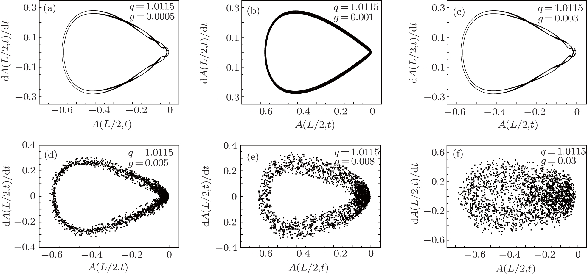
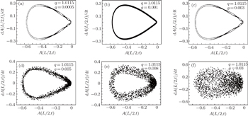
For q = 1.0115 and different quintic parameter g, the phase trajectories are shown in Fig. 6. A motion of two-loop can be observed in Fig. 6(a) for g = 0.0005 and we believe that the pseudorecurrence appears. As g increases further, the trajectory becomes a single loop that starts from and goes back to the same saddle (A,A_t) = (0,0), which forms the Kolmogorov–Arnold–Moser (KAM) torus. The KAM torus becomes very thick for g = 0.001 as presented in Fig. 6(b). When g = 0.003, the two-loop structure corresponds to pseudorecurrence is observed again in Fig. 6(c). With the increase of g, the pseudorecurrence breaks down again as shown in Figs. 6(d)–6(f) for g ≥ 0.005, which indicates the appearance of the temporal chaos. From Fig. 6, we conclude that the changing process is as follows for q = 1.0115 and increasing g: the pseudorecurrence with two-loop → the quasirecurrence which forms the KAM torus → the pseudorecurrence with two-loop again → the stochastic motion or irregular motion.

Fig. 6.

	Figure Option ViewDownloadNew Window
	Fig. 6. Phase trajectories of the cubic–quintic NSE by symplectic method with θ = 45.18°, q = 1.0115, and different parameter g: (a) g = 0.0005, (b) g = 0.001, (c) g = 0.003, (d) g = 0.005, (e) g = 0.008, (f) g = 0.03.

The dynamic behaviors of the cubic–quintic NSE with different cubic and quintic nonlinear parameters are studied by the symplectic scheme. Numerical results show that the conserved quantities are well preserved and our method is reliable. For different cubic parameters, the system will exhibit various properties with the increase of the quintic nonlinear parameter, and these properties are illustrated by the phase trajectories, the time evolution of the amplitude of the wave, and the corresponding Fourier spectrum. When q = 0.01, the trajectory in phase space is an elliptic orbit and the origin is an elliptic point. When q is increased to q = 0.75, the trajectory in phase space is a homoclinic orbit (HMO), and will become an elliptic orbit with the increase of g. When we further increase the cubic parameter to q ≥ 0.925, the system exhibits more complex properties with the increase of g which may lead to regular or irregular HMO crossings, and the motion of the system will change from the periodic recurrence to the pseudorecurrence and to chaos. In conclusion, the changing processes are various for different cubic nonlinear parameters with the increase of the quintic nonlinear parameter. The basic dynamic behaviors of the cubic–quintic NSE are very important in several branches of physics and mathematics, and it is very significant to study the behaviors of the cubic–quintic NSE with different nonlinearity.