As an important branch of network science, synchronization of complex networks has been paid great attention and studied deeply in the past two decades. It is well known that synchronization plays an important role in various fields, such as laser systems, communication systems, and parallel image processing.^[1–6] In the research of complex dynamical networks, a variety of synchronization patterns have been defined and studied, including complete synchronization,^[7] partial synchronization,^[8] cluster synchronization,^[9,10] projective synchronization,^[11] phase synchronization,^[12] lag synchronization (LS),^[13] generalized synchronization,^[14] etc. Among these patterns, the LS between two coupled systems has been studied extensively.^[15–17]

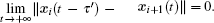
Most existing researches of LS are based on two coupled dynamical systems (or networks). The LS is achieved if y(t) → x(t − τ), τ > 0 as t → + ∞, which is investigated originally in Ref. [13]. From then on, LS has gradually become a research focus. The LS has been generalized to many other forms, including projective lag synchronization,^[18] generalized lag synchronization^[19] and successive lag synchronization (SLS).^[20] Here, SLS, a new kind of lag synchronization in a multi-coupled dynamical system proposed by Li in Ref. [20], can be considered as a generalized pattern of the traditional LS in two coupled systems. SLS means that a node achieves the LS with its next node, i.e., x_i(t − τ) → x_i+1(t) for a positive time delay τ as t → +∞. It may be found potential applications of SLS in multi-agent systems. For example, in military parade, sometimes we can see that the aircrafts (nodes) pass the same spatial position with the same time delay to avoid collision and keep orderly queue, which can be considered as the SLS realization of these aircrafts. In Ref. [20], the authors supposed that there is no communication delay between nodes in the network means that each node in the network can immediately receive the coupling signals from its neighbor nodes. However, because of the finiteness of signal transmission and switching speed, the communication delay is inevitable in real dynamical systems.^[21] Communication delay often appears in numerous systems frequently, such as aircraft, seismology, and laser systems.

Motivated by the above discussions, the main aim of this paper is to construct a general dynamical network with communication delay and investigate its SLS. Based on the constructed dynamical network, we apply linear feedback control and adaptive control to achieve its SLS. Depending on topological structure of the considered dynamical network, a linear feedback control is designed to realize its SLS. Moreover, in order to choose the feasible control adaptively, an adaptive linear feedback control is also proposed. By using the Lyapunov function method and Barbalat’s Lemma, some sufficient conditions for the global stability of SLS are obtained.

The rest of this paper is organized as follows. In Section 2, we give some Lemmas and some preliminaries about the model formulation of a dynamical network with communication delay. In Section 3, we investigate the global stability conditions of the SLS of the dynamical network under linear feedback control and adaptive linear feedback control, respectively. In Section 4, some numerical examples are performed to verify the theoretical results. Finally, in Section 5, we conclude the paper.

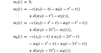
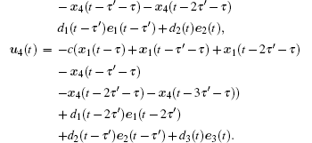
The considered dynamical network with communication delay under control is described as follows:

Definition 1^[20] Successive lag synchronization (SLS) of dynamical network is said to be achieved if, for any initial condition and every i ∈ {1,2,…,n − 1},

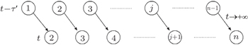
It should be noticed that we should first number the nodes in a network according to the Definition 1 to prepare for the study of its certain SLS. The schematic figure of SLS is shown in Fig. 1.

Fig. 1.

	Figure Option ViewDownloadNew Window
	Fig. 1. The schematic figure of successive lag synchronization in a network with size n.

Definition 2^[22] Function class QUAD (Δ,P,ω): let a diagonal matrix Δ = diag{δ₁,δ₂,…,δ_m} and a positive-definite diagonal matrix P = diag{p₁,p₂,…,p_m}. QUAD(Δ,P,ω) denotes a class of continuous functions f(x,t) : ℝ^m × [0,+∞) → ℝ^m satisfying

Lemma 1^[23] For a matrix M = (m_ij)_p×q, the inequality

From Barbalat’s Lemma, Li gives the following result in Ref. [20].

Lemma 2 If g(t): ℝ → ℝ⁺ is a uniformly continuous function for t ≥ 0 and if the integral

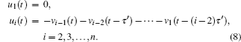
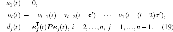
In order to eliminate suppressive items in the following error system (10) and accelerate the realization of SLS, we design the following preliminary functions and control. First, for i = 1,2,…,n − 1, some preliminary functions are defined as

Then a linear feedback control can be designed as

According to Definition 1, the SLS errors of dynamical network (1) are defined as e_i(t) = x_i(t − τ′) − x_i+1(t) for i = 1,2,…,n − 1. Then the error system can be described as

Theorem 1 Let Δ = diag{δ₁,δ₂,…,δ_m} be diagonal matrix and P = diag{p₁,p₂,…,p_m} be positive-definite diagonal matrix, such that f(x) ∈ QUAD(Δ,P). If there exists d > 0 such that

Proof Define the following Lyapunov functional candidate:

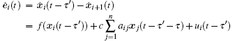
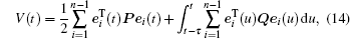
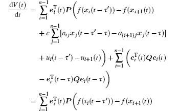
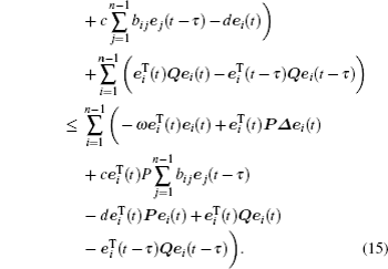
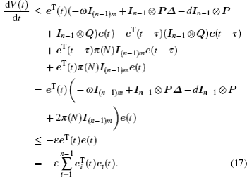
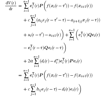
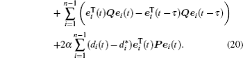
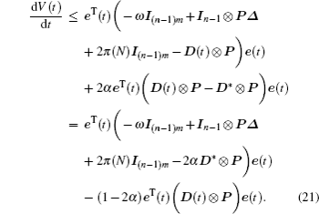
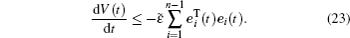
The derivative of V(t) along the trajectories of error system (10) can be obtained as follows:

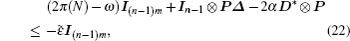
Letting , from Eq. (15), we obtain

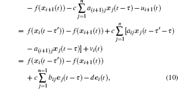
From condition (13), there exists a constant ɛ > 0 such that (2π(N) − ω)I_(n−1)m + I_n−1 ⊗ PΔ − dI_n−1 ⊗ P ≤ − ɛI_(n−1)m. From Lemma 1, letting N = cB ⊗ P, we obtain

Integrating the above equation from 0 to t yields

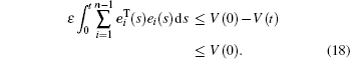
Thus, the integral is bounded. From Lemma 2, we obtain for every i ∈ {1,2,…,n − 1}, which means that This completes the proof.

In practice, the control strength is not allowed to be arbitrarily large, so we adopt an adaptive control method^[22] to reduce the control strength.

For i = 1,2,…,n − 1, some preliminary functions are similarly defined as

Then an adaptive control is designed as

Suppose that Δ = diag{δ₁,δ₂,…,δ_m} is a diagonal matrix and P = diag{p₁,p₂,…,p_m} is a positive-definite diagonal matrix. Then we have the following result under adaptive control (19).

Theorem 2 If f(x) ∈ QUAD(Δ,P), then the SLS of dynamical network (1) can be achieved for any initial conditions under adaptive control (19).

Proof Define the following Lyapunov functional candidate:

The derivative of V(t) along trajectories of error system (10) is calculated as follows:

Thus, the integral is bounded. From Lemma 2, we obtain for every i ∈ {1,2,…,n − 1}, which means that This theorem is proven.

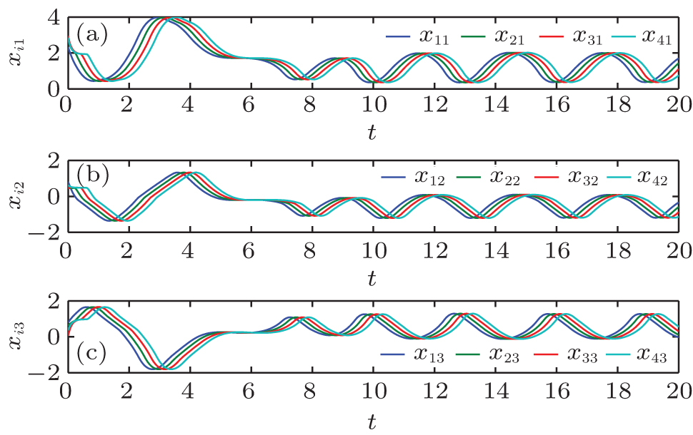
In this section, some numerical examples are given to verify the theorems in Section 3. The size of dynamical network (1) is set as n = 4 and its topological structure is shown in Fig. 2 with two cases. The local dynamics of all nodes in this network is characterized by a 3D neural network,^[9] which is described by

Fig. 2.

	Figure Option ViewDownloadNew Window
	Fig. 2. Two kinds of topological structure for dynamical network (1) with size n = 4. (a) Loop-shaped network; (b) fully connected network.

4.1. Linear feedback control

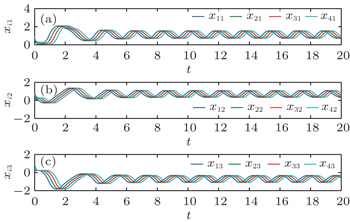
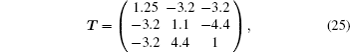
First, we use linear feedback control (8) to realize SLS on a dynamical network, whose topological structure is shown in Fig. 2(a). The coupling matrix of this network structure is

From Eqs. (11) and (12), we obtain

According to control (8), we have

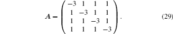
We can obtain π(N) = (n − 1)m × max_ij{|n_ij|}/2 = 9c from the matrix B. In order to achieve (13), we choose c = 0.1 and search the lower bound of the control strength d by solving the following inequality:

We can easily get the lower bound of the control strength d_l = 11.18. So, if d > d_l, the conditions of Theorem 1 are satisfied, which means that the SLS of dynamical network (1) under control (8) can be achieved for any initial conditions. Figure 3 gives a realization under control strength d = 12 and time delay τ = 0.5, and figure 5 shows its SLS errors on the same condition. From these simulations, we can see that the SLS is achieved under linear feedback control (8). In order to explore the influence of communication delay on the SLS, we change τ to 1 and obtain Fig. 4. This realization is under control strength d = 12, which shows that SLS is still achieved. Hence, the stability condition is independent on communication delay.

Fig. 3.

	Figure Option ViewDownloadNew Window
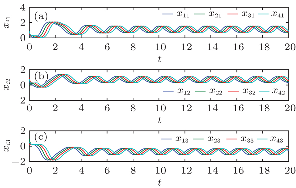	Fig. 3. Trajectories of (a) xi1, (b) xi2, and (c) xi3 of dynamical network (1) under control (8), where i = 1,2,3,4, c = 0.1, d = 12, τ′ = 0.2, and τ = 0.5.

Fig. 4.

	Figure Option ViewDownloadNew Window
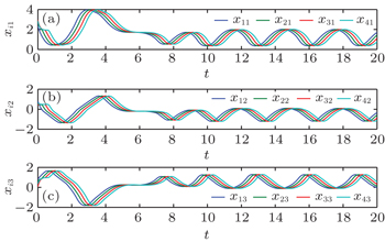
	Fig. 4. Trajectories of (a) xi1, (b) xi2, and (c) xi3 of dynamical network (1) under control (8), where i = 1,2,3,4, c = 0.1, d = 12, τ′ = 0.2, and τ = 1.

Fig. 5.

	Figure Option ViewDownloadNew Window
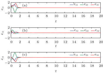
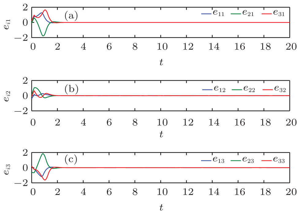
	Fig. 5. Trajectories of SLS errors (a) ei1, (b) ei2, and (c) ei3 of dynamical network (1) under control (8), where i = 1,2,3, c = 0.1, d = 12, τ′ = 0.2, and τ = 0.5.

4.2. Adaptive linear feedback control

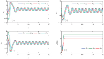
Now, we use adaptive control (19) to realize SLS on another dynamical network, whose topological structure is shown in Fig. 2(b). The coupling matrix of this network is

According to adaptive linear feedback control (19), we have

Figure 6 presents a realization under adaptive linear feedback control (19) with coupling strength c = 0.1 and τ′ = 0.2 and τ = 0.5. Figure 7 gives the errors. As shown in Figs. 6 and 7, we can see that the SLS of dynamical network (1) is achieved under adaptive linear feedback control (19).

Fig. 6.

	Figure Option ViewDownloadNew Window
	Fig. 6. Trajectories of all state variables (a) xi1, (b) xi2, (c) xi3, and (d) di(t) of dynamical network (1) under control (19), where i = 1,2,3,4, c = 0.1, τ′ = 0.2, and τ = 0.5.

Fig. 7.

	Figure Option ViewDownloadNew Window
	Fig. 7. Trajectories of all SLS errors (a) ei1, (b) ei2, and (c) ei3 of dynamical network (1) under control (19), where i = 1,2,3, c = 0.1, τ′ = 0.2, and τ = 0.5.

Similar to that in subsection 4.1, by solving the following inequality:

we gain the lower bound of the control strength d_l = 12.08. As shown in Fig. 6, we can observe that all control strengths are obviously smaller than d_l, which confirms that the adaptive linear feedback control can decrease the control strength required for the realization of SLS.

In this paper, we address the successive lag synchronization (SLS) on dynamical networks with communication delay via linear feedback control and adaptive linear feedback control. We construct a general dynamical network with communication delay to make the SLS more realistic and significant for real multi-coupled systems. By using the linear feedback control, the SLS of the network has been realized. In order to choose the feasible control gain adaptively, we design an adaptive linear feedback control. By theoretical analysis, we obtained some sufficient conditions for the global stability of SLS under the controls.

In many real dynamical networks, their topological structures may be generally directed. Therefore, it is worth to consider SLS of dynamical networks with directed topological structures in the future.