The Mott–Hubbard metal-insulator transition (MIT)^[1] caused by electron–electron interaction is one of the central issues in the physics of strongly correlated electron systems. A variety of many-body methods such as dynamical mean-field theory (DMFT)^[2,3] have been developed to study the transitions in models and realistic materials. Till now, most of the model studies on MIT are focused on the single band Hubbard model, which has been viewed as the “Hydrogen atom" for MIT. However, in most of the realistic materials, the transition should be described by multi-band Hubbard models and the transition is greatly influenced by the fluctuation of electrons among different orbitals, which is absent in the simple single band model. As a consequence, the physics of MIT in multi-band systems is much richer with many exotic phenomena occurring, i.e., the orbital-selective Mott transition (OSMT).^[4]

The OSMT was first introduced to explain the complicated behavior of conduction electrons in Ca_{2 − x}Sr_xRuO₄,^[4] where at least part of the conduction electrons are itinerant while the rest seem to be localized. Since then, a lot of model studies have been carried out to uncover the mechanism of OSMT. Firstly, a two-band Hubbard model with different band widths at half-filling has been investigated by different groups.^[5–14] In this case, electrons are equally distributed within the two bands. With the increment of Coulomb interaction U, two different bands undergo MIT separately. The band with narrower band width becomes Mott insulator first due to its stronger correlation strength while the one with wider band width still remains metallic, indicating an OSMT. Those studies also confirm that the Hund’s coupling, both the Ising-type^[7,10] (only J_z is considered) and the rotational invariant type^{[5–9,13,14]} (including spin-flip J_s and pair-hopping J_p terms), plays a very important role in OSMT. Secondly, OSMT can exist in a three-band Hubbard model with equal band width in the presence of crystal field splitting (CFS) at integer filling 2, 3, or 4. The average filling of four electrons per site was studied in detail by de’Medici et al. in Ref. [15]. In their model, one orbital is lifted by the CFS, while the other two orbitals keep degenerate. They find a large orbital-selective Mott phase (OSMP) region in the phase diagram and large Hund’s coupling can enlarge the OSMP region as a “band decoupler”. The case of two electrons per site in a three-band Hubbard model has been studied by Kita et al. in Ref. [16] and they find an OSMT region in the phase diagram at large Hund’s coupling. Thirdly, doping-driven OSMT has also been studied by some groups.^[17–23] In the case of two-band Hubbard model with different band widths, OSMT can still be stable away from half-filling in certain parameters region.^[17–19] Werner et al.^[20] have considered a two-band Hubbard model with equal band width split by crystal field. They find that, in the presence of CFS, doping would first drive one of the bands into metallic phase while leaving the other one in a Mott phase, thus inducing the OSMT. Further doping would drive the other band into metallic phase. In this case, the underlying physics to drive an OSMT is doping. However, the physics behind such a doping-induced OSMT with equal band width has not been studied in detail yet, which inspires the current study.

In this paper, we will focus on the detailed physical aspects of doping-driven OSMT. We consider a multi-band Hubbard model with equal band width, in which the CFS lifts one of the bands to higher energy (upper band) and leaves the other bands (lower bands) to be degenerate. Through the DMFT calculations, we will show that in such a system we can find a doping-induced OSMT, which is very surprising because usually doping electrons will turn the Mott phase into the metallic phase or the opposite.

We start from the situation where the lower bands are half-filled and the upper band is forced to be empty by adjusting the CFS. Suppose that at the beginning the system is near the critical point of MIT but still in the metallic side. Then, we start to dope electrons into the upper band but still keep the lower bands half-filled by tuning the CFS properly. We find that there will be a critical doping point, after which the lower half-filled bands will be driven into a Mott phase while the upper band still keeps the metallic phase within a considerable region of the CFS. We also find that further increasing doping concentration will enlarge the OSMP region. Finally, we reach the critical doping concentration at which both the upper and the lower bands are half-filled, and the OSMP merges into a single Mott phase. Therefore, we realize a doping-driven OSMT in multi-band systems in the presence of CFS. The systems described above can be realized by both two-band and three-band Hubbard models. In this paper, both models are studied in detail by the DMFT method combined with the high precision hybridization expansion continuous time quantum Monte Carlo (HYB-CTQMC) impurity solver.^[24–26] The phase diagram as a function of total electron filling N and CFS Δ are calculated. Based on the results, we summarize this mechanism of OSMT as: (i) with strong Hund’s coupling, doping electrons to a multi-band system with special CFS will help to form and stabilize the local magnetic moment; (ii) large local magnetic moment will scatter electrons strongly and enhance the effective correlation strength, which will cause a Mott transition in some certain bands, thus leading to an OSMT.

We consider the following multi-band Hubbard model defined as^[27]

We can solve this lattice model defined in Eq. (1) in the framework of single-site DMFT,^[2,3] which ignores the momentum dependence of the self-energy and maps the lattice model into an effective impurity model being solved self-consistently. We use a semicircular density of states, , which corresponds to the infinite-coordination Bethe lattice, where D = 2t is the half band width and all bands keep equal band width. To solve the effective impurity problem, we use the HYB-CTQMC impurity solver^[24–26] implemented in the iQIST package,^[28] which allows us to access the strong interaction regime down to very low temperature. The temperature is set to be T = t/40 (corresponding to the inverse temperature βt = 40) through all our calculations. In each DMFT iteration, we have typically performed 2 × 10⁸ QMC samplings to reach sufficient numerical accuracy.

Now, we will first focus on the two-band case. To demonstrate the OSMT when doping the system, we have calculated the phase diagram as a function of the total electron filling N and the CFS Δ. The electron filling per orbital per spin, spin–spin correlation function χ(τ) and the effective local magnetic moments M^z,eff as a function of the CFS for various N are also calculated to understand the phase diagram. Based on these results, we will show the importance of doping which drives and stabilizes the OSMT.

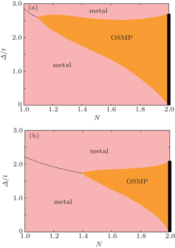
The calculated N–Δ phase diagram is shown in Fig. 1. The Coulomb interaction is set to be U/t = 4.90 and two different Hund’s coupling values are considered: J_z = 0.25U (Fig. 1(a)) and J_z = 0.20U (Fig. 1(b)). We choose this value of Coulomb interaction in order to make the system at the critical point of MIT, and of course, other values of U can also give very similar phase diagram, only with different phase boundaries. We calculate the quasiparticle weight by to determine the phase for each orbital, where ω₀ = π/β and Σ_α(iω_n) is the self-energy function. It is metallic when Z_α is finite and it is Mott phase when Z_α approaches to zero. Except for the metallic phase in the pink region, we find a large OSMP region (orange area) and this region is extended at larger Hund’s coupling. The black dashed line indicates the state in which the lower orbital is half-filled but still metallic and the black bar at N = 2 indicates that both orbitals are half-filled and in a Mott phase.

Fig. 1.

Figure Option ViewDownloadNew Window

Fig. 1. The phase diagram as a function of the total electron filling N and the crystal field splitting Δ for the two-band Hubbard model with Ising-type Hund’s coupling, U/t = 4.90, (a) Jz = 0.25U and (b) Jz = 0.20U. The orange area denotes the orbital-selective Mott phase, where the lower orbital is in a Mott phase while the upper orbital is metallic. The pink area denotes that both orbitals are metallic. The black dashed line denotes that the lower orbital is half-filled but still metallic. The black bar at N = 2 indicates that both orbitals are half-filled and in a Mott phase.

To understand the phase diagram, we plot the redistribution of electrons when increasing the CFS at a fixed total electron filling N, the results for U/t = 4.90, J_z = 0.25U are shown in Fig. 2. We take N = 1.50 for example. Initially, in the absence of the CFS, the electrons distribute equally within the two orbitals. If we continuously increase Δ, the electrons will gradually populate into the lower orbital until it is half-filled (indicated by the left blue arrow in Fig. 2). After that, further increasing the CFS will not populate more electrons into the lower orbital because it will pay a higher energy cost due to the strong Coulomb interaction among the electrons in the lower orbital. As a result, the system may come into a state, in which the lower orbital always keeps half-filling (the plateau between the blue arrows in Fig. 2) in a considerable region of the CFS. We also find that this plateau will reach earlier at large doping (see N = 1.90 for example, plateau indicated by the green arrows). On the contrary, for very small doping (for example N = 1.05), we cannot see an obvious plateau. Therefore, the plateau becomes wider when doping is larger. However, if the CFS is large enough (comparable with U), the electrons will again populate into the lower orbital to avoid the cost of the large CFS energy.

Fig. 2.

	Figure Option ViewDownloadNew Window
	Fig. 2. The electron filling per orbital per spin as a function of the crystal field splitting Δ for three selected total electron filling N = 1.05, 1.50, 1.90, respectively. Here, U/t = 4.90, Jz = 0.25U. Note that the upper orbital is marked as “orb1" and the lower orbital is marked as “orb2”.

Based on the knowledge about the redistribution of electrons discussed above, we can understand the whole phase diagram. The metallic phase in pink region can be understood easily because both of the orbitals are away from the condition of half-filling. The most interesting part of the phase diagram is the metallic phase indicated by the black dashed line and the OSMP in the orange region. The black dashed line represents the state in which the lower orbital is half-filled but metallic. On the contrary, in the orange area, the lower orbital is also half-filled but it is in a Mott phase, and as a whole the system is in an OSMP. These facts remind us that the lower half-filled orbital should have undergone a MIT when the doping becomes larger and the MIT has strong connection with the plateau of electron filling. Actually, as mentioned above, when the filling of the lower orbital continues to increase to be half-filled by increasing the CFS, the rest of the doped electrons will fill the upper orbital, and these electrons will interact with the electrons in the lower orbital through the strong Hund’s coupling to help to form total local magnetic moments and stabilize them. The more doped electrons, the larger magnetic moments and it means that the system favors a high-spin state (HS)^[20] when doping becomes large.

To illustrate this, we calculate the spin–spin correlation function and the effective local magnetic moments. The spin–spin correlation function^[29–31] can be used to describe the dynamical screening of the local magnetic moments, which is defined as

Fig. 3.

	Figure Option ViewDownloadNew Window
	Fig. 3. The spin–spin correlation function χ(τ) as a function of imaginary time τ from 0 to β/2 at U/t = 4.90, Jz = 0.25U. Here, (a) N = 1.50, Δ/t = 2.0, in OSMP phase, (b) N = 1.05, Δ/t = 2.7, in metallic phase. In both cases, the lower orbital is half-filled. χ11(τ), χ22(τ), χtot(τ) are for upper orbital, lower orbital, and total contributions, respectively.

Fig. 4.

Figure Option ViewDownloadNew Window

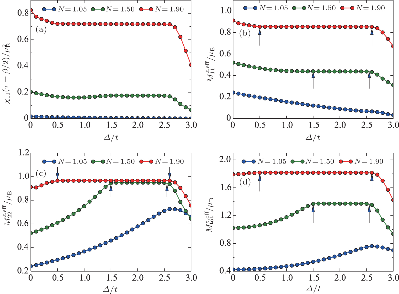Fig. 4. Spin–spin correlation function and effective local magnetic moments as a function of crystal field splitting Δ for N = 1.05, 1.50, 1.90 at U/t = 4.90, Jz = 0.25U. (a) The spin–spin correlation function at τ = β/2 for upper orbital χ11(τ = β/2), (b) the effective local magnetic moments for upper orbital , (c) the effective local magnetic moments for lower orbital , (d) the total effective local magnetic moments . The arrows indicate plateaus.

In the presence of large local magnetic moments, the charge fluctuation will be suppressed because the electrons will be scattered by the local magnetic moments. As a result, the effective Coulomb correlation strength U_eff of the lower half-filled orbital will be enhanced when increasing doping, after a critical value , the lower orbital will undergo a MIT and an OSMT occurs. In summary, the more doping, the larger local magnetic moments and the wider OSMP region, and the OSMT occurs as long as the electron filling per orbital comes into the plateau. In the OSMP region, the itinerant electrons of the upper orbital will show non-Fermi liquid (NFL) behavior.^[29] This is due to the scattering by the large total local magnetic moments, including the contribution of local moments in the lower insulating band and the frozen moments in the upper metallic band. At N = 2.0, the upper orbital also undergoes a MIT, as a whole, the system is in the Mott phase, which is illustrated as the black bar in Fig. 1. Here, we should emphasize that the Hund’s coupling plays a crucial role. We can see that the OSMP region for J_z = 0.20U is smaller than that for J_z = 0.25U. Thus, large Hund’s coupling is a prerequisite for OSMT, which is consistent with the conclusion of previous studies.^{[5–10,13,14]}

Next, we discuss the case of three-band Hubbard model with Ising-type Hund’s coupling. In this case, two orbitals keep degenerate and another orbital is lifted by the CFS. The N–Δ phase diagram at U/t = 2.80, J_z = 0.25U is shown in Fig. 5. The main character of this phase diagram is very similar to that of the two-band model and the mechanism of OSMT does not change. The OSMT occurs when the lower two orbitals are half-filled and the doping is large enough. It seems that the OSMP region is smaller than that of the two-band case, actually, this is due to the choice of the Coulomb interaction U and Hund’s coupling J_z.

Fig. 5.

Figure Option ViewDownloadNew Window

Fig. 5. The phase diagram as a function of the total electron filling N and the crystal field splitting Δ for the three-band Hubbard model with Ising-type Hund’s rule coupling at U/t = 2.80, Jz = 0.25U. The orange area denotes the orbital-selective Mott phase where the lower two orbitals are in a Mott phase while the upper orbital is metallic. The pink area denotes that all orbitals are metallic. The black dashed line indicates that the lower two orbitals are half-filled but still metallic. The black bar at N = 3 indicates that all the three orbitals are half-filled and in a Mott phase.

Finally, we would emphasize the difference between this mechanism of OSMT and previous studies^[17–19] of the OSMT in doped multi-band Hubbard models. In their studies, the bands have different band widths, so the effective Coulomb interaction strength is different for each band, which may lead to an OSMT. However, in our study, we do not need the condition of different band widths, and the effective Coulomb interaction strength of the lower bands will be enhanced by the local magnetic moments which are formed and stabilized by the doping electrons of the upper band, thus leading to an OSMT.

In summary, we have found a doping-driven OSMT in multi-band Hubbard model with equal band width in the presence of the CFS. When the Hund’s coupling is large enough, the doped electrons in the upper orbital will help to form large local magnetic moments which will scatter electrons and suppress the charge fluctuation, thus the effective correlation strength of the lower orbitals will increase large enough to undergo an MIT. In such a way, an OSMT occurs. The more doping, the more stable OSMP. This mechanism of OSMT can be realized in both two-band Hubbard model and three-band Hubbard model with Ising-type and rotational invariant Hund’s coupling. We hope that this mechanism of OSMT can also be found in some realistic strongly correlated metallic materials.