Project supported by the National Natural Science Foundation of China (Grant No. 11404255) and the Doctor Foundation of Education Ministry of China (Grant No. 20130201120013).
Abstract
Abstract
The second-order temporal interference of two independent single-mode continuous-wave lasers is discussed by employing two-photon interference in Feynman’s path integral theory. It is concluded that whether the second-order temporal interference pattern can or cannot be retrieved via two-photon coincidence counting rate is dependent on the resolution time of the detection system and the frequency difference between these two lasers. Two identical and tunable single-mode continuous-wave diode lasers are employed to verify the predictions. These studies are helpful to understand the physics of two-photon interference with photons of different spectra.
In Feynman’s point of view, interference is at the heart of quantum physics and it contains the only mystery of quantum physics.[1] It should be helpful to understand quantum physics if interference is understood better. Interference can be divided into different categories based on different criteria. For instance, based on the source employed, interference can be categorized into interference with sound waves, photons, massive particles, etc. Based on the order, interference can be categorized into the first-, second-, third-, and high-order interference. Based on the valid superposition principle, interference can be categorized into quantum interference and classical interference.[2] Among all kinds of interference mentioned above, two-photon interference is an ideal tool to study the properties of interference in quantum physics besides single-photon interference. The reasons are as follows. Two-photon interference is a second-order interference phenomenon, which is the simplest higher-order interference of light. Photon is a quantum concept and two-photon interference belongs to quantum interference.[2,3] The interference experiments with photons are much easier than the ones with massive particles, so that the theoretical predictions can be verified conveniently.
Two-photon interference, which is also known as the second-order interference of light, was first observed by Hanbury and Twiss in 1956, in which they found that randomly emitted photons by thermal light source arrive at two detectors in bunches rather than randomly.[4] Theoretical explanations for this strange phenomenon advance the development of optical coherence theory. Among all the interpretations, Glauber’s quantum optical coherence theory may be the most successful one, which is usually thought as the foundation of modern quantum optics.[5,6] In Glauber’s quantum optical theory, two-photon bunching of thermal light can be understood by two-photon interference.[7] Two-photon interference has been studied extensively with photons in both classical and nonclassical states[8–10] since the observation of two-photon bunching of thermal light.[4] Recently, two-photon interference with photons of different spectra has drown lots of attention due to its possible applications in quantum information processing.[11–22] All the experiments did not take the resolution time of the detection system into account except Ref. [17], in which Flagg et al. pointed out that the observed dip is affected by the response time of the detector. In the recent experiments about the second-order interference of two independent lasers,[21,22] the influence of the resolution time on the observed interference pattern is not considered, either. In this paper, we will study in detail how the resolution time of the detection system affects the observed second-order interference pattern when the frequency difference between these two lasers varies. Two independent and tunable single-mode continuous-wave lasers are employed to verify theoretical predictions. We will also discuss the physics of two-photon interference with photons of different spectra, which is helpful to understand the physics of interference.
The organization of the following parts is as follows. In Section 2, we will theoretically study the second-order temporal interference of lasers with different spectra based on the superposition principle in Feynman’s path integral theory. The second-order interference experiments with two independent and tunable single-mode continuous-wave diode lasers are described in Section 3. The discussion and conclusions are given in Sections 4 and 5, respectively.
2. Theory
Although the second-order interference of classical light can be interpreted by both quantum and classical theories,[5,6,23] we will employ two-photon interference based on the superposition principle in Feynman’s path integral theory to interpret the second-order interference of two independent lasers with different spectra. Recently, we have employed this method to discuss the second-order subwavelength interference of light,[24] the spatial second-order interference of two independent thermal light beams,[25] the second-order interference between thermal and laser light,[26] etc. These studies indicate that the advantages of this method are not only simple, but also offer a unified interpretation for all orders of interference with photons in both classical and nonclassical states. The scheme in Fig. 1 is employed in the following calculations.
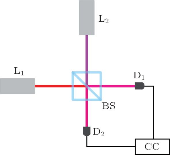
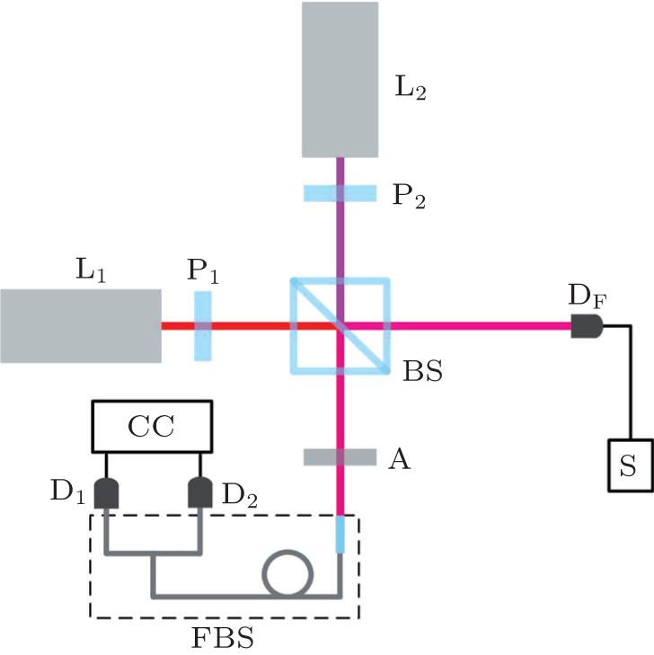
Fig. 1. Second-order interference of two independent lasers. Two independent laser light beams are incident to two adjacent input ports of a 1:1 non-polarizing beam splitter (BS), respectively. L1 and L2 are two single-mode continuous-wave lasers. D1 and D2 are two single-photon detectors. CC is two-photon coincidence count detection system. The mean frequencies of photons emitted by L1 and L2 are ν1 and ν2, respectively. The distance between the laser and detection planes are all equal. For simplicity, the polarizations and intensities of these two light beams are assumed to be identical, respectively.
There are three different cases to trigger a two-photon coincidence count in Fig. 1. (i) Both photons are emitted by L1. (ii) Both photons are emitted by L2. (iii) One photon is emitted by L1 and the other photon is emitted by L2. Although the frequencies of the photons emitted by these two lasers are different, the photons are indistinguishable if |ν1 − ν2| is less than 1/Δtu, where Δtu is the time measurement uncertainty of photon detection.[3,27] Photon is usually detected by photoelectric effect in a single-photon detector. It has been proved by Forrester et al. that the time delay between photon absorption and electron release is significantly less than 10−10 s,[28] which can be treated as the time measurement uncertainty.
When photons emitted by these two lasers are indistinguishable, the two-photon probability distribution for the j-th detected photon pair is[24,29]
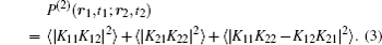
where φL1 and φL2 are the phases of photons emitted by L1 and L2 in the j-th detected photon pair, respectively; Kαβ is the Feynman’s photon propagator from Lα to Dβ at (rβ,tβ) (α, β = 1, 2). The extra phase π/2 is due to the photon reflected by a beam splitter will gain an extra phase comparing to the transmitted one.[30] The final two-photon probability distribution is the sum of all the two-photon probability distributions,
where 〈···〉 is ensemble average by taking all the two-photon probability distributions into consideration. Since L1 and L2 are independent, 〈ei (φL1−φL2)〉 equals 0. Equation (2) can be simplified as
The first and second terms on the right-hand side of Eq. (3) correspond to two-photon coincidence counts of photons emitted by L1 and L2, respectively. The third term on the right-hand side of Eq. (3) corresponds to two-photon interference when two photons are emitted by two lasers, respectively. In order to simplify the calculations, we assume that the modes of both lasers are plane wave. Feynman’s photon propagator for a photon in the plane wave is[31]
which is the same as Green function in classical optics.[32]kαβ and rαβ are the wave and position vectors of the photon emitted by Lα and detected at Dβ, respectively. να and tβ are the frequency and time for the photon that is emitted by Lα and detected at Dβ, respectively (α, β = 1, 2).
Substituting Eq. (4) into Eq. (3) and with similar calculations to that in Refs. [10], [22] and [24]–[26], it is straightforward to have one-dimensional temporal two-photon probability distribution as
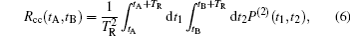
where paraxial and quasi-monochromatic approximations have been employed to simplify the calculations. The positions of D1 and D2 are assumed to be the same in order to concentrate on the temporal part. Δν is the frequency difference between these two lasers, which equals |ν1 − ν2|. The maximum visibility is 50%, which is consistent with the conclusion in Ref. [33]. Two-photon coincidence counting rate is[8,34,35]
where TR is the resolution time of two-photon detection system. With a similar method used in Refs. [10] and [35] and setting τ+ = (t1 + t2)/2, τ− = t1 − t2, equation (6) can be simplified as
where cos[2πΔν(t1 − t2)] = Re{exp(2πΔν(t1 − t2))} has been employed in the calculation. sinc(x) equals sinx/x. Based on Eq. (7), we can discuss the relationship between the measured two-photon coincidence counting rate and two-photon probability distribution function in three different situations.
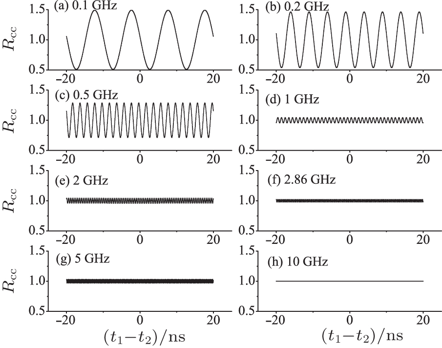
In this regime, the observed two-photon coincidence counting rate is proportional to the two-photon probability distribution function modulated by a sinc function. In order to get an intuitive understanding about the relationship between two-photon coincidence counting rate and two-photon probability distribution function, figure 2 presents the simulated two-photon coincidence counting rates for different values of frequency difference. The parameters are similar to the ones in our experiments in order to compare the theoretical and experimental results. The central wavelength of the laser is 780 nm. The frequency bandwidth is 100 kHz. The resolution time of the detection system is 0.35 ns. The time window for the second-order temporal interference pattern is 40 ns and the time width for each channel is 0.0122 ns. Figures 2(a)–2(h) correspond to the frequency differences between these two lasers are 0.1, 0.2, 0.5, 1, 2, 2.86, 5, 10 GHz, respectively. When the frequency difference is 0.1 GHz, the beating period is 10 ns. The resolution time of the detection system is much less than the beating period. The observed two-photon coincidence counting rate is the same as two-photon probability distribution function, where the visibility is 50% as shown in Fig. 2(a). The visibility of the observed interference pattern decreases as the frequency difference between these two lasers increases, which can be seen from Figs. 2(a)–2(e). In Fig. 2(f), the resolution time equals the inverse of the frequency difference between these two lasers. It is almost impossible to retrieve the interference pattern from two-photon coincidence counting rate. However, if we analyze the simulated two-photon coincidence counting rate closely, the second-order interference pattern still exists. The reason why there seems no interference pattern is the visibility is 2.22%. When the frequency difference is 10 GHz, the visibility is 0.02%, in which no two-photon interference pattern can be observed via two-photon coincidence counting rate.
Fig. 2. Simulated two-photon coincidence counting rates when the frequency difference varies. Rcc: two-photon coincidence counting rate. t1 − t2: time difference between two single-photon detection event for a two-photon coincidence count. The parameters for the simulation are as follows. Central wavlength: 780 nm, frequency bandwidth: 100 kHz, resolution time: 0.35 ns, channel width: 0.0122 ns. Time window: 40 ns. (a)–(h) correspond to the frequency difference between these two lasers are 0.1, 0.2 0.5, 1, 2, 2.86, 5, 10 GHz, respectively.
However, it should be noted that the simulations in Fig. 2 is based on Eq. (7), which is valid when the frequency difference is less than 1/Δtu. Photons with frequency difference larger than 1/Δtu are distinguishable. Probabilities instead of probability amplitudes should be added to get the j-th detected two-photon probability distribution in Eq. (1).[1,29] In this condition, equation (3) should be changed into
in which no second-order interference pattern exists in the two-photon probability distribution.
When a fiber beam splitter is put at one output of BS to measure the second-order temporal interference pattern as the one in Fig. 3, only the positions of phase factor, π/2, change in Eq. (1). With the same method above, two-photon coincidence counting rate (Eq. (7)) is changed into
It is easy to find that equations (7) and (10) are identical except that the minus sign in Eq. (7) is changed into plus sign in Eq. (10). All the discussion above is valid for the scheme in Fig. 3.
Fig. 3. Experimental setup for the second-order interference of two tunable single-mode lasers. L1 and L2 are two identical grating stabilized tunable single-mode diode lasers (DL100, Toptica Photonics). The central wavelength and frequency bandwidth of the laser are 780 nm and 100 kHz, respectively. P1 and P2 are two linearly polarizers to ensure that the polarizations of these two light beams are identical. DF is a fast amplified silicon detector (ET-2030A, Electro-Optics Technology, Inc.). S is a spectrum analyzer (Agilent E441B) to monitor the frequency difference between these two lasers. D1 and D2 are two single-photon detectors (SPCM-AQRH-14-FC, Excelitas Technologies) and CC is two-photon coincidence counting system (SPC630, Becker & Hickl GmbH). BS is a 1:1 non-polarizing beam splitter. A is an optical attenuator to decrease the intensity of light so that the single-photon counting rates of both detectors are around 50000 c/s. FBS is a 1:1 non-polarizing fiber beam splitter, which is employed to ensure that the positions of these two detectors are identical. The optical distance between the laser and DF is equal to the one between the laser and the collector of FBS, which is 525 mm. The length of FBS is 2 m.
3. Experiments
In Section 2, we have calculated two-photon probability distribution and coincidence counting rate in the second-order interference of two independent single-mode continuous-wave lasers with different spectra. In this section, we will employ the experimental setup in Fig. 3 to verify our predictions.
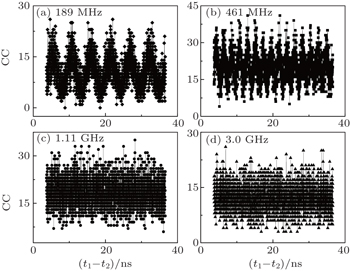
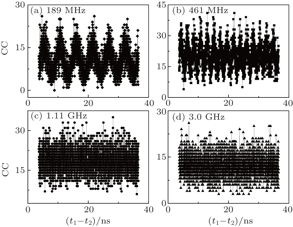
The measured two-photon coincidence counts are shown in Fig. 4. The dark counts of both single-photon detectors are less than 100 c/s. CC is two-photon coincidence count. t1 − t2 is the time difference between these two single-photon detection events within a two-photon coincidence count. Each two-photon coincidence counting rate in Fig. 4 is collected for 120 s. The measured coincidence counts are raw data without subtracting any background. The second-order interference pattern is observed in Fig. 4(a), in which the frequency difference is 189 MHz. The beating period is 5.29 ns, which is larger than the resolution time of our detection system, 0.35 ns. The frequency difference between these two lasers is varied by tuning the frequency of L2 while fixing the frequency of L1. When the frequency difference is 461 MHz, the second-order interference pattern can also be observed as shown in Fig. 4(b). The visibility of the interference pattern in Fig. 4(b) is less than the one in Fig. 4(a). No interference pattern is observed in Fig. 4(c), in which the frequency difference is 1.11 GHz. Although there is interference pattern in the simulation in Fig. 2(d) when the frequency difference is 1 GHz. It is difficult to retrieve the interference pattern experimentally via two-photon coincidence counting measurement due to its low visibility. When the frequency difference is 3 GHz, there is no second-order interference pattern observed in Fig. 4(d), either. The observed experimental results in Fig. 4 are consistent with the theoretical predictions in Fig. 2.
Fig. 4. Measured two-photon coincidence counts when the frequency difference is (a) 189 MHz, (b) 461 MHz, (c) 1.11 GHz, () 3.0 GHz. CC: two-photon coincidence count. t1 − t2: time difference between two single-photon detection event for a two-photon coincidence count. The collection time for each figure is 120 s.
4. Discussion
In the last two sections, we have calculated the second-order temporal interference pattern of two independent single-mode continuous-wave lasers when the frequency difference varies and employed two tunable lasers to verify the theoretical predictions. The reason why the observed interference patterns are different when the frequency difference varies is dependent on the resolution time of the detection system and the frequency difference. When the resolution time is much less than the beating period, the observed two-photon coincidence counting rate is identical to the two-photon probability distribution function. The visibility of the observed interference pattern decreases as the frequency difference increases, which has been confirmed both theoretically and experimentally in Figs. 2 and 4, respectively. When the frequency difference is larger than a certain value, the visibility of two-photon coincidence counting rates approaches 0. The interference pattern cannot be observed.
It is worth noting that although the second-order interference pattern cannot be observed when the frequency difference exceeds a certain value in our experiments, the second-order interference pattern still exists when the frequency difference is less than 1/Δtu. There is interference pattern in the simulation when the frequency difference is 2 GHz in Fig. 2(e). The second-order interference pattern can be retrieved if we have a detection system with much shorter resolution time. Based on the discussion above, a question arises naturally. Is it possible to observe two-photon interference between any photons if we have a detection system with infinity small resolution time? The answer is yes in classical physics for there is no limit on the measurement accuracy. In quantum physics, the answer is no since the measurement accuracy is limited by Heisenber’s uncertainty principle.[2,27] The time measurement uncertainty in photon detection is determined by the photon detection mechanism. In the photon detection based on photoelectric effect, the time measurement uncertainty is significantly less than 10−10 s.[28] Without loss of generality, we assume the time measurement uncertainty of photon detection based on photoelectric effect is 10−10 s. Photons with frequency difference larger than 10 GHz is distinguishable for the detection system.[29] The different ways to trigger a two-photon coincidence count are distinguishable in the scheme in Fig. 1. Based on the superposition principle in Feynman’s path integral theory,[1,29] there is no two-photon interference when different alternatives are distinguishable. Two-photon probability distribution is given by Eq. (9) when the frequency difference is larger than 10 GHz. No second-order interference pattern exists in this condition.
It is well-known that the observed result is dependent on the measuring apparatus in quantum physics. For instance, there is no two-photon interference for photons with frequency difference larger than 10 GHz if the detection system based on photoelectric effect is employed. It does not mean there is no two-photon interference for other detection systems. For instance, the time measurement uncertainty of two-photon absorption is at 10−15 s range.[36] Photons with frequency difference less than 106 GHz are indistinguishable. There is two-photon interference when the frequency difference is less than 106 GHz for detection system based on two-photon absorption. Photons with different spectra are distinguishable for some detection systems, while these photons can be indistinguishable for other detection systems. When talking about the measured results in quantum physics, one has to pay special attention to the employed measuring apparatus.[37]
Although our calculations and experiments are for the second-order interference of classical light. The discussion and conclusions above can be generalized to the second-order interference of nonclassical light.[11,12,14–17,20] For instance, when these two lasers are replaced by two single-photon sources in Fig. 1, there are only two possible alternatives to trigger a two-photon coincidence count. One is the photon emitted by source 1 goes to detector 1 and the photon emitted by source 2 goes to detector 2. The other alternative is the photon emitted by source 1 goes to detector 2 and the photon emitted by source 2 goes to detector 1. The same method as the one in Section 2 can be employed to calculate the second-order interference of photons in nonclassical states. Furthermore, the method is also valid for the second-order interference between classical and nonclassical light. For instance, there is two-photon interference by superposing photons emitted by laser and nonclassical light source if the photons are indistinguishable for the detection system.[38]
5. Conclusions
In conclusion, we have theoretically and experimentally studied the second-order temporal interference of two independent single-mode continuous-wave lasers when the frequency difference varies. Whether the second-order interference pattern can be retrieved via two-photon coincidence counting measurements is dependent on the resolution time of the detection system and the frequency difference of these two superposed lasers. When the resolution time is much less than the beating period, the observed two-photon coincidence counting rate is the same as two-photon probability distribution function. When the resolution time of the detection system is fixed, the visibility of the observed second-order interference pattern decreases from 50% to nearly zero as the frequency difference increases. When the frequency difference is larger than the inverse of time measurement uncertainty of the detection system, there is no two-photon interference for the different alternatives to trigger a two-photon coincidence count are distinguishable. The results are helpful to understand the second-order interference of light in the languages of photons.
Reference
1
FeynmanR PLeightonR BSandsM L2004The Feynman Lectures on PhysicsVol. IIIBeijingBeijing World Publishing Corp.
2
DiracP A M1958The Princinples of Quantum Mechanics4th edn.OxfordOxford University Press


 , Chen Hui1, 2, Zhou Yu3, Zheng Huaibin1, 2, 3, Gao Hong3, Li Fu-Li3, Xu Zhuo1, 2]