

A cellular automaton model for the ventricular myocardium considering the layer structure
[Deng Min-Yi† , Dai Jing-Yu, Zhang Xue-Liang]
, Dai Jing-Yu, Zhang Xue-Liang]
|
|


†Corresponding author. E-mail: dengminyi@mailbox.gxnu.edu.cn
*Project supported by the National Natural Science Foundation of China (Grant Nos. 11365003 and 11165004).
A cellular automaton model for the ventricular myocardium considering the layer structure has been established. The three types of cells in this model differ principally in the repolarization characteristics. For the normal travelling waves in this model, the computer simulation results show the R, S, and T waves and they are qualitatively in agreement with the standard electrocardiograph. Phenomena such as the potential decline of point J and segment ST and the rise of the potential line after the T wave appear when the ischemia occurs in the endocardium. The spiral wave has also been simulated, and the corresponding potential has a lower amplitude, higher frequency, and wider R wave, which accords with the distinguishing feature of the clinical electrocardiograph. Mechanisms underlying the above phenomena are analyzed briefly.
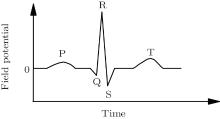
The ventricle is one of the most important parts of the heart. The ventricle beats with high speed when ventricular fibrillation happens, which may result in sudden death, [1] so the dynamics of the transmembrane potential of the ventricle has received much attention.[2– 5] The QRS complex and T wave of electrocardiograph (ECG) are the collective reflection of the ventricular electronic activity (Fig. 1).[6] The depolarization and repolarization of the ventricle are responsible for the QRS complex and T wave, respectively. On the temporal morphology of the standard ECG, the T wave is the first up wave after the QRS complex, where the potential is positive.[6] Myocardial diseases can usually be diagnosed with ECG; especially, the arrhythmia cannot be diagnosed without ECG. So the relation between the ECG and the electric activity of the myocardium cells should be made clear. Experiment is the main method used to study the electric activity of the myocardium cells on the macroscopic level. For example, based on a quasi-two-dimensional layer of the left ventricular epicardium of a white rabbit, Veniamin et al. studied the transition between the damped waves and the steadily propagating waves in the cardiac tissue.[2] Using the data of a patient who suffered from regular and sudden-onset fast palpitation, Sorgente et al. researched the contribution of the T wave vector in localizing the site of origin of the ventricular tachycardia.[4] But until now, no experimental reports about the relation between the myocardial electric activation and the ECG on the cellular level can be found. The reason for this may be the huge number of myocardial cells. The numerical simulation models play an important assistant role in exploring this relation. The numerical simulation models of myocardial electrical activation are classified into two major groups: one is the reaction– diffusion model, and the other is the cellular automaton (CA) model. Studies based on the former have obtained remarkable results about the dynamics of the spirals in excitable media.[7– 10] In this paper, a CA model is established to recovery the relation between the cellular electric activation and the ECG.
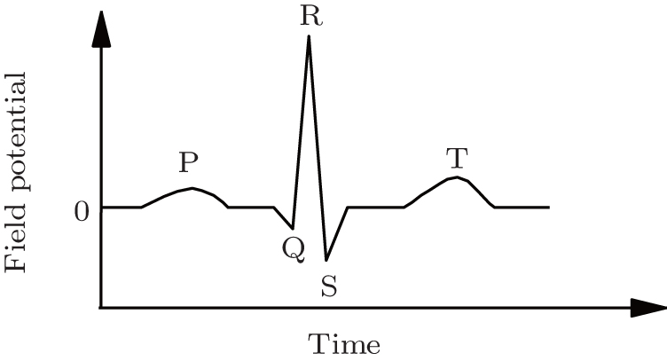 | Fig. 1. The standard ECG.[6] |
CA is a simple and effective numerical method.[11] The CA approach usually oversimplifies the real system, but as long as the rules keep the basic properties of the system, we can still learn many interesting facts and gain insights into the mechanism underlying the phenomena.[12] Because of the easy realization of the program and the high speed of computation, CA has been used in the study of cardiac tissue for decades. For example, CA models for atrial tissue, [13] ventricular tissue, [3] and the sinoatrial node[14] have been established. Some researchers have also studied the electric signal of cardiac cells with CA. For example, Mitchell et al. performed a theoretical analysis of ventricular fibrillation and the requirements for fibrillation.[15] Zhu et al. studied the electric activity of the heart with a CA system.[16, 17] However, the CA model in Ref. [3] did not consider the layer structure of the real ventricle, and the CA system in Refs. [16] and [17] contained the complex ionic currents, which violates the principle of simplification of CA. Consequently, t is necessary to establish a new CA model for the ventricle tissue.
In this paper, a CA model for the ventricle tissue considering the three-layer structure is reported. There are three types of cells in this CA model. The computer simulation is carried out. The results show the R, S, and T waves when the system evolves with the electric travelling waves under the normal conditions. In the case of an ischemia happening in the endocardium, the point J and the segment ST decline, while the potential line after the T wave rises. The spiral-wave state of the electric impulse and the corresponding electrogram are also simulated. In the following sections, the model, the simulation results, and the conclusion will be presented.
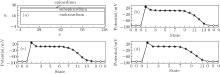
The experimental results have demonstrated three types of cells in the ventricular wall: endocardial, subepicardial, and epicardial cells.[18] These three types of cells have different repolarization characteristics: the action potential duration (APD) of the subepicardial cells is the longest; however, the deference between the epicardial cells and the endocardial cells is not worthy of mention.[19] On the other hand, the endocardium is the thickest, then the subepicardium, and the epicardium is the thinnest.[18] Considering the above factors, we construct the CA model for the ventricle as follows: the ventricle slice is put on the xoy coordinate surface, where the y axis direction is from endocarium to epicardium (Fig. 2(a)). This two-dimensional ventricle slice is divided into 128 × 32 sites. The ventricular cells are distributed on these sites. According to the thicknesses of the cells, the endocardium, subepicardium, and epicardium occupy 25 sites, 5 sites, and 2 sites, respectively. The transmembrane potential of a cell can be in m states. The state of cell (x, y) at discrete time t is represented by ux, y (t) ∈ (0, 1, 2, … , m − 1) with m ≥ 3. The ux, y (t) = 0, 1 denotes the rest and the excited states, respectively, while ux, y (t) = 2, … , m − 1 represents the refractory states. Obviously, the APD of a cell equals m − 1. Referring to Ref. [19], the different types of cell have different m; for example, m in this paper is 14, 15, and 12 for endocardial, subepicardial, and epicardial cells, respectively (Figs. 2(b)– 2(d)).
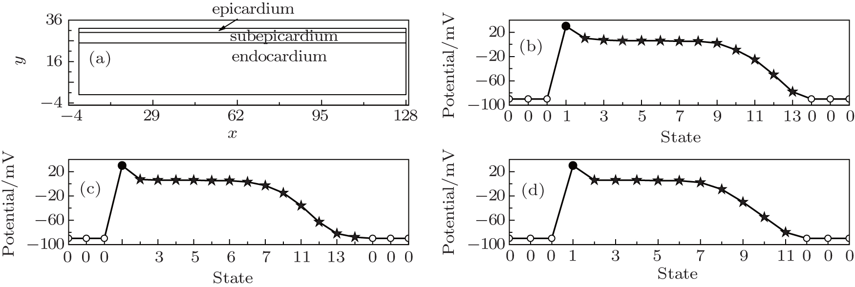 | Fig. 2. CA model for a ventricle slice. (a) Ventricle slice containing three layers. Transmembrane potentials of (b) endocardial cells, (c) subepicardial cells, (d) epicardial cells. Symbols ∘ , • , and ★ represent the rest, the excited, and the refractory states, respectively. |
The no-flux boundary condition and the Moore neighborhood are used throughout this paper. For radius r, there are (2r + 1)2 − 1 neighbors in a cell’ s neighborhood. If the number of excited neighbors of cell (x, y) at time t is n, then the time evolution of the cell is given as follows:
where K is the excitable threshold.
When the computer simulation is done, the potential at the field point is calculated using the formula proposed by Zhu et al.[17]

where σ in = 1.28 S/m is the intracellular conductivity; [20]S0 is a constant that just affects the baseliner, and here S0 = 32; N is the total number of the cells; there are eight nearest neighbors of each cell; Vi is the transmembrane potential of the i-th cell in the system; Vj is the transmembrane potential of the j-th neighbor of the i-th cell; θ j is the included angle between two directions: one points from the i-th cell to its j-th neighbor, the other points from the j-th neighbor of the i-th cell to the field point; σ i is the average conductivity of the cells along the direction from the i-th cell to the field point; and, rj is the distance from the j-th neighbor of the i-th cell to the field point. For simplicity, we let the conductivity of the other medium besides the cardiac cells be 0.74 S/m.[20]
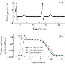
The electric impulse is produced at the sino-atrial node, and then transmits to the atria, the atrioventricular node, and finally to the ventricle.[21] Because of the properties of the conduction system in the ventricle, the impulse can spread throughout the ventricle in a short time.[21] To imitate this physiological characteristic, all of the endocardial cells are set at the excited state initially (t = 0), while the other cells are set at the rest state. Let r = 5, which makes sure that the subepicardium can be excited in one step, and then the epicardiaum. After three steps, the system returns to the refractory states. According to the difference of APD between these three types of cells, the epicardial cells first come back to the refractory states, and then the endocardial cells, and finally the subepicardial cells. At last, the system returns to the rest state. The system will repeat the above state transformation again as long as the endocardial cells accept other impulses. The excitable threshold is K = 2, the period of impulse is Te = 33, and the field point is (130, 40), which is close to the V4 lead of the electrocardiographic leads.[6] The simulated potential trajectory is shown in Fig. 3(a). To analyze the mechanism underlying the trajectory in Fig. 3(a), the simultaneously recorded transmembrane potentials from endocardial, subepicardial, and epicardial cells are shown in Fig. 3(b).
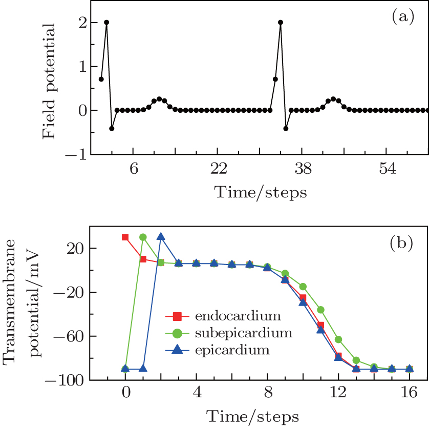 | Fig. 3. (a) Electrogram recorded at (130, 40) and (b) the simultaneously recorded transmembrane potentials from endocardium, subepicardium, and epicardium cells, where K = 2, r = 5, and Te = 33. |
By comparing Fig. 3(a) with Fig. 1, we find that the potential trajectory shows the typical R, S, and T waves when the electric impulse evolves as a travelling wave in the ventricle slice. The occurrence mechanism of these waves can be found in Fig. 3(b). According to Eq. (1), the potential comes from the differences of the transmembrane potentials; in our CA model, it comes from the differences of the transmembrane potentials of the three types of cells. For example, at the first step (t = 0), only the endocardial cells are excited, so the transmembrane potential of the endocardial cells is higher than that of the subepicardial cells, which contributes a positive potential to the field point (see the point at t = 0 in Fig. 3(a)). The other points in Fig. 3(a) can be analyzed similarly. It is necessary to point out the significance of the T wave. According to the definition of the T wave, one can find in Fig. 3(a) that the first T wave starts at t = 7 and ends at t = 15. In Fig. 3(b), the potential differences between the three layers hardly exist between these two moments without the existence of the subepicardium. So the existence of the subepicardium is the foundation of the T wave, which is a well-known physiological conclusion.[19] The ventricle slice considered here does not include the ventricular septum, which is responsible for the Q wave according to the physiological version, [6] so the Q wave does not appear here.
The segment ST is an iso-electric level which starts at the end of the S wave and ends before the start of the T wave; [6] for example, the segment in Fig. 3(a) starts at t = 3 and ends at t = 7. The point J is the first point of the segment ST, [6] the point is at t = 3 in Fig. 3(a). The potentials of segment ST and point J will decline when the ischemia occurs in endocardium.[6] To simulate this phenomenon, we suppose that the region within x = 120 to x = 128 and y = 0 to y = 25 is ischemic. The cells in the ischemic region act with higher resting potential and shorter APD[22] compared with that of the normal cells (Fig. 4(a)). The simulated potential trajectory is shown in Fig. 4(b).
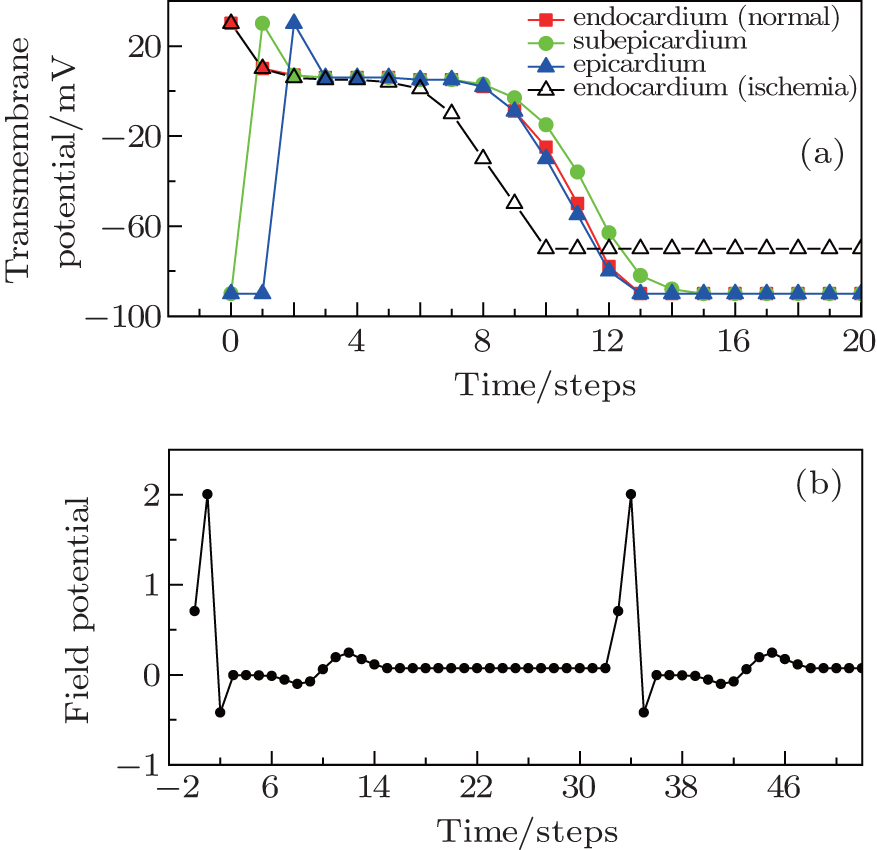 | Fig. 4. (a) Simultaneously recorded transmembrane potentials from endocardium, subepicardium, and epicardium; and (b) electrogram recorded at (130, 40). Parameters are the same as those in Fig. 3 except the existence of the ischemia in endocardium. |
The results in Fig. 4(b) show that: (i) the potentials of point J and segment ST really decline. For example, the potential at t = 3 (the first point J) is no longer 0 in Fig. 3(a) but − 0.0036, and the potential reduces continuously afterwards until it reaches the minimum − 0.1035 at t = 8. Because of the shorter APD, the transmembrane potential of the ischemia endocardial cells is much smaller than that under the normal conditions between these two moments, which results in the even more negative potential for the field point (130, 40). (ii) The potential line after the T wave raises; for example, the potential between t = 15 and t = 32 in Fig. 4(b) is 0.0722, but it is 0 in Fig. 3(a). These results can be explained with Fig. 4(a): between t = 15 and t = 32, because of the higher resting potential, the transmembrane potential of the ischemia endocardial cells is no longer equal to but larger than that of the subepicardial cells, which contributes a positive potential to the field point (130, 40), and then results in the rise of that potential line.
Nasha et al. indicated that many dangerous cardiac arrhythmias may come from the spiral wave state of the cardiac electric impulse, and fibrillation appears once the spiral wave state turns into the turbulence state.[23] The spiral wave is a self-sustained wave state. When the excitation spreading along the longside of an infinitely inhomogeneous stripe is cut, the stationary propagation of a wave segment can be observed.[24] But in the ventricle CA model used here, the impulse spreads across the longside of the slice, which makes it impossible to produce a spiral wave under the normal conditions: the electric impulse spreads very fast under the normal conditions, so even the travelling wave is cut, the cut-down point goes out off the system quickly, and then the spiral wave state cannot come into being. Pathological changes will reduce the conduction ability of the conduction system in the ventricle.[21] On the other hand, the decrease of the excitation ability can also reduce the wave speed. To imitate these two situations, only the endocardial cells within y ≤ 5 are set at the excited state initially (t = 0), and the value of K is no longer 2 but is now 14. The other parameters are the same as those in Fig. 3. When the computer simulation is done, the travelling wave is cut down at t = 6 (Fig. 5(a)). The results show that when the cut-down point returns to the endocardium, the endocardial cells have come back to the rest state, so the impulse can spread continually, and the spiral wave finally comes into being (Figs. 5(b) and 5(c)). The further computer simulation results indicate that if there is no more impulse coming from the endocardium, then the spiral wave will be maintained for ever. The potential at field point (130, 40) is recorded again, and the results are shown in Fig. 5(d).
 | Fig. 5. Distributions of the excited state at (a) t = 6, (b) t = 14, (c) t = 139, the black represents the excited state; (d) the electrogram recorded at (130, 40). The parameters are the same as those in Fig. 3, except K = 14. |
Figure 5(d) indicates that when the impulse evolves with spiral state, the potential trajectory appears as follows: (i) the amplitude of the potential is 0.5447, which is much smaller then 2.0039 in Fig. 3(a) under the normal conditions; (ii) the period of the potential is 15 steps, not 33 steps in Fig. 3(a) under the normal conditions; and, (iii) the wide R wave appears, which corresponds to the clinic ECG as the ventricular tachycardia occurs.[6] The last two phenomena have been observed in the clinic.[4] So the above results support the conclusion that the spiral wave state may be the reason for the ventricular tachycardia.
In this paper, a CA model considering the three-layer structure is proposed for a ventricle slice. Three types of cells with characteristic repolarization properties are distributed on the three layers. The computer simulation results exhibit the following phenomena. (i) Under normal conditions, the R, S, and T waves appear in the potential trajectory, which corresponds to the standard ECG. This result agrees with the physiological conclusion about the existence of the subepicardium. (ii) When the ischemia occurs in the endocardium, the potential decline of point J and segment ST and the raise of the potential line after the T wave can be observed, which is close to the clinic conclusion. This result comes from the shorter APD and higher resting potential of the ischemia cells in endocardium. (iii) When the impulse evolves with the spiral-wave state, the potential trajectory has a smaller amplitude, shorter period, and wide R wave, which supports the conclusion that the spiral-wave state maybe the reason for the ventricular tachycardia. The above phenomena indicate that the CA model in this paper is appropriate for the ventricle slice, and the work has reference value for further study in the dynamics of the electric impulse of the cardiac.
| 1 |
|
| 2 |
|
| 3 |
|
| 4 |
|
| 5 |
|
| 6 |
|
| 7 |
|
| 8 |
|
| 9 |
|
| 10 |
|
| 11 |
|
| 12 |
|
| 13 |
|
| 14 |
|
| 15 |
|
| 16 |
|
| 17 |
|
| 18 |
|
| 19 |
|
| 20 |
|
| 21 |
|
| 22 |
|
| 23 |
|
| 24 |
|