

Strong violations of locality by testing Bell’s inequality with improved entangled-photon systems
[Wang Yaoa) , Fan Dai-Hea) , Guo Wei-Jiea) , Wei Lian-Fu†a), b)  ]
]
]
|
|


†Corresponding author. E-mail: weilianfu@gmail.com
*Project supported by the National Natural Science Foundation of China (Grant Nos. 61308008, 91321104, U1330201, and 11174373) and the Fundamental Research Funds for the Central Universities (Grant No. 2682014CX081).
Bell’s theorem states that quantum mechanics cannot be accounted for by any local theory. One of the examples is the existence of quantum non-locality is essentially violated by the local Bell’s inequality. Therefore, the violation of Bell’s inequality (BI) has been regarded as one of the robust evidences of quantum mechanics. Until now, BI has been tested by many experiments, but the maximal violation (i.e., Cirel’son limit) has never been achieved. By improving the design of entangled sources and optimizing the measurement settings, in this work we report the stronger violations of the Clauser–Horne–Shimony–Holt (CHSH)-type Bell’s inequality. The biggest value of Bell’s function in our experiment reaches to a significant one: S = 2.772± 0.063, approaching to the so-called Cirel’son limit in which the Bell function value is
In 1935, Einstein, Podolsky, and Rosen (EPR) queried the completeness of quantum mechanics and believed that the nonlocal correlation in the quantum world should be caused by the incompleteness of quantum theory.[1] To complete the quantum mechanics, the so-called hidden-variables theory was introduced.[2, 3] In the framework of the hidden-variables theory, the nonlocal correlation is regarded as the induction of a certain local feature. In 1964, Bell proposed an inequality to test the validity of the hidden-variables theory, and proved that the predictions of quantum theory are incompatible with those of any physical theory satisfying the natural notion of locality.[4]
It is well known that the nonlocal quantum mechanics has being used in many fields, such as quantum communication, quantum computation, and so on.[5] For example, Resch et al., [6] distributed the polarization-entangled photons over a distance of 7.8 km and showed that high-fidelity transfer of entangled photons is possible. This provides the promise for the future quantum communication using satellites. Imaginably, the quantum non-locality will take an increasingly important role in various quantum technologies.
Physically, the experiment is the best evidence for any theorem. Therefore, many experiments have been done to test the violation of Bell’ s theorem since 1964. Until now, many forms of the Bell inequality have been proposed but CHSH’ s type[7] is the easiest to experimentally test.[8, 9] Note that almost all of the previous experiments supported the results which violate the Bell inequality, and the result opposite to quantum mechanics was owed the technologic error in the experiments. In particular, from 1980s laser physics and modern optics changed the experiment pattern. By nonlinear laser excitations of an atomic radiative cascade, the quality of the used entangled sources have been enhanced significantly and thus Bell’ s theorem can be tested more robustly. Typically, in 1981 Aspect et al.[10– 12] successfully tested Bell’ s theorem by checking the violations of three forms of Bell’ s inequality, including the CHSH one.[10] The measured value of the CHSH function is S = 2.697 ± 0.015 with the standard deviations being greater than 40. This proved that the CHSH inequality was violated in a sufficiently high confidence coefficient, although the loop-hole in the non-locality still exists. Up to the late 1980s, with the technology of the parameter down-conversion for generating entangled-photon pairs and the optical fiber for achieving the nonlocal measurements, the local loop-hole could be closed for testing the quantum non-locality. First, relevant experiments for testing Bell’ s inequality using the polarized entanglements of the photons generated by parameter down-conversions were first performed by Ou and Mandel, [13] Shih and Alley, [14] and the CHSH function S = 2.21 ± 0.022 was obtained by Rarity and Tapster.[15] Later, better results, e.g., S = 2.6489 ± 0.0064, [16] 2.7007 ± 0.0029, [17] and 2.7277 ± 0.0719, [18] were obtained successively in experiments. Next, with the help of optical fiber technology, Aspelmeyer et al.[19] implemented a long distance (about 600 m) experiment to test the CHSH inequality and the relevant CHSH function S = 2.41 ± 0.10 was measured. In 2005, Peng et al.[20, 21] further realized the test of CHSH inequality with the entangled photons distributed by a 13-km long free space and the measured CHSH function is S = 2.45 ± 0.09. In principle, the longer distance means the larger loss of the entangled photons, and thus limits the larger value of the CHSH function. Anyway, the biggest violation of the BI, i.e, the CHSH function reaches to the Cirel’ son limit:[22]
By improving the quality of the entangled sources and optimizing the relevant measurement settings, we show in this paper that the stronger violation of the CHSH inequality can be realized. Our work focuses on the two lacks in the usual experiments for testing the BI. First, the usual entangled sources utilized are practically not the ideal maximal entangled states and also not in the pure states. Second, the used measurement settings corresponding to the pure-state assumption are not suitable for experiments. Therefore, in our experiments we not only optimize the entangled sources by filtering various stray lights but also optimize the measurement settings based on the tomographic constructions of the states. As a consequence, we demonstrated the optimal violation of the CHSH inequality, i.e., the CHSH function reaches S = 2.772 ± 0.063, approaching further the Cirel’ son limit.
This paper is organized as follows. In Section 2, we introduce our experimental system and discuss how to improve the quality of the entangled sources by checking the relevant polarization correlation curve between the photons generated by pumping the BBO crystal. With the quantum tomographic technique, [23] in Section 3 we first find out the optimized measurement settings accordingly, and then perform the test of CHSH inequality. Section 4 is our summary.
Based on EPR’ s arguments and Bell’ s logic, if the physical quantities, a and b, of two uninteracting systems separated spatially are independent and each of them takes only two values: E(α ) = 1 (α = a, b), or E(α ) = − 1, then the existence of the so-called hidden variable λ (with ∫ ρ (λ )dλ = 1) implies that E(α , λ ) = ± 1. Here, the distribution function ρ (λ ) of a hidden variable is independent of α . Considering the uncertainty and error in the practical measurement, we have: |E(a, λ )E(b, λ )| ≤ 1. Thus, for the correlation function

of the two measured systems, one can easily prove that

Consequently, the well-known CHSH inequality

which will be tested experimentally. Specifically, for the usual polarization-entangled photon-pair systems the local polarization information is selected as the measured polarization directions α , β of the two photons. Therefore, the measurable CHSH function reads

with α , α ′ and β , β ′ being the local variables of the entangled two photons, respectively. Experimentally, the correlation function E(α , β ) can be determined as

where P(α , β ) is the photon coincidence counts for one photon being detected along the α -angle polarization and another along the β -angle polarization.
Suppose we have a pure-state entangled-photon source

with θ , φ being two controllable parameters, then the measurement settings of the two photons can be selected as
As a consequence, the photon coincidence counts should be
Especially, for θ = π /4, φ = 0, π we get

and thus

Therefore, if the measurement settings are selected as (α , α ′ , β , β ′ ) = (− 45° , 0° , − 22.5° , 22.5° ), then the CHSH function reaches its maximum value: 
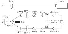
Figure 1 is our experimental setup. The used semiconductor laser is a commercial product[24] with the power of 95 mW and the central wavelength of 405 nm. A nonlinear type-I down-conversion medium (bulk beta-barium borate (BBO)) crystal is utilized to generate the desirable entangled-photon pairs. The detection system of each photon constitutes a detector, a polarization beam splitter (PBS), and a half wave plate (HWP). The filters are used to strain the stray light. Finally, the counter shows the coincidence signal of the two detectors.
 | Fig. 1. The experimental setup. The lens is used to converge the laser beam, HWPs are used to adjust the polarizations of photons, the BBO crystal down-converts the pump light. The quarter-wave plate (QWP) adjusts the phase position for tomographically reconstructing the density matrix of the generated entangled source. An HWP, a PBS (polarization beam splitter), and an avalanche diode detector form a polarization measurement system of the photon. The filters are introduced to strain the stray light. Finally, the counter shows the coincidence signals of the two detectors. |
Experimentally, the polarization of the photon out of the laser is vertical, i.e., |V〉 -polarization. The angle of the first HWP is set as 45° , such that the polarization of the photon after the HWP is changed as 45° . The entangled photons are generated by pumping the I-type BBO crystal, see Fig. 2. Here, the BBO crystal is formed by two nonlinear crystals with orthometric crystal axis. Under the phase matching and the energy conservation conditions, the entangled photons will appear at the symmetric positions. As the thickness of the BBO crystal is sufficiently thin, the two light cones produced by the BBO crystal can be treated as coincident light. Thus, the generated entangled source can be described by the following pure state

 | Fig. 2. Parameter down-conversion of the laser via an I-type BBO crystal. |
To mark the quality of the generated entangle source, we measure the relevant polarization correlation curves. Ideally, the generated entangled-photon state should be coherently superposed purely by the state |H〉 |H〉 and |V〉 |V〉 . But, in practice, the photons are in the unwanted states |H〉 |V〉 and |V〉 |H〉 . Therefore, the measured coincidence counts corresponding to the |H〉 |H〉 and |V〉 |V〉 should be far significantly greater than those to the |H〉 |V〉 and |V〉 |H〉 states. In addition, we need to eliminate the situation corresponding to the mixed state superposed by |H〉 |H〉 and |V〉 |V〉 . This can be achieved by performing alternatively the |± 〉 -measurement; 
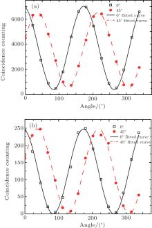
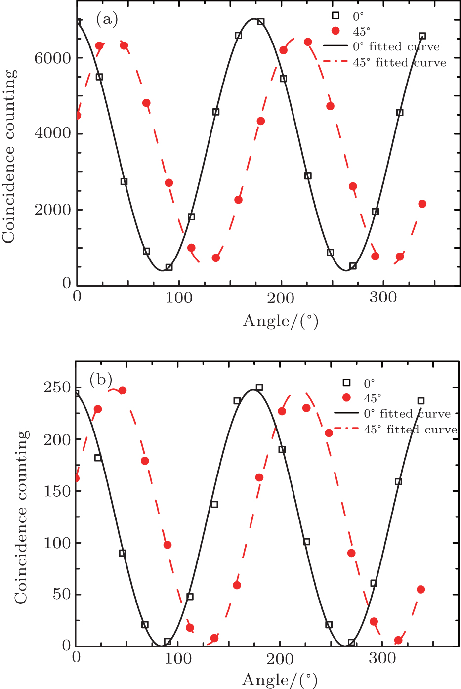 | Fig. 3. The polarization correlation curve: panel (a) is the image with a pair of long-pass filters; and panel (b) is the image with a pair of interference filters. Here, the black squares represent the counts which are measured by the |H〉 -polarization in the first path and 22.5° -polarization in the other path, and the black full line is the fitted curve by the black squares; the red dots represent the counts which are measured by the |+ 〉 -polarization in the first path and 22.5° -polarization in the other path, and the red dotted line is the fitted curve by the red dots. It is observed that the latter induces the better quality. |
Phenomenally, a parameter

can be introduced to mark the quality of the entangled source with, e.g., the CHH being the coincidence counts for the measuring settings |H〉 |H〉 -polarization (i.e., both of the photons are measured at the |H〉 -polarizations). Note that, ξ = 0.8457 in Fig. 3(a), wherein the long-pass filter is used; but ξ = 0.9609 is obtained in Fig. 3(b), wherein an interference filter is used. This indicates that the quality of the entangled source can be obviously enhanced by introducing the interference filters.
With the polarization entangled-photon pairs demonstrated above, we now test the CHSH inequality by properly designing the measurement settings to determined the value of the CHSH function S ± σ with the experimental statistical uncertainty σ s. Experimentally, by directly reading out the coincidence counts n(α , β ) of the two detectors for the local variables α , β , we have the relevant coincidence probabilities

Then, from Eq. (5), the correlation function E(α , β ) can be directly calculated as

Therefore, to obtain the CHSH functions we need to measure the correlation fucntions: E(α , β ), E(α ′ , β ), E(α , β ′ ), and E(α ′ , β ′ ). From Eq. (13), one can see that four coincidence counts are required to be detected for each correlation function, and thus we need to detect 16 coincidence counts, ni (i = 1, 2, 3, 4, … , 16) to determine the value of the CHSH function. Here, the statistical uncertainty σ s can be calculated as

where, the coincidence counts are considered as the Poisson statistical distribution, and thus the standard deviation σ ni for each coincidence counts is 
Primarily, one imagines that the entangled source is the desirable maximally entangled state, and performs the test for the optimized local variables: (α , α ′ , β , β ′ ) = (− 45° , 0° , − 22.5° , 22.5° ). The results of the detections are listed in Table 1. With these data, the values of the CHSH function for the above primary tests are obtained:
| Table 1. Experimental data of the coincidence counts obtained by the measurement settings (α , α ′ , β , β ′ ): L corresponds to the using of long-pass filters, and F represents the using of interference filters. |
Given the entangled-source fixed, we now investigate how to enhance the degree of violation of the BI. In the above primary tests, we assumed that the entangled-source is the maximally entanglement of the generated photon pairs. Correspondingly, the measurement settings are naturally set as (α , α ′ , β , β ′ ) = (− 45° , 0° , − 22.5° , 22.5° ). However, the realistic entangled-source should not be the exactly maximally-entangled state. This implies that the measurement settings used above for the primary tests should be adjusted accordingly.
First, the entangled-source generated should be characterized by the quantum-state tomograph technique.[23] For the present two-qubits system, the density matrix ρ of the entangled-source can be generically expressed as[25]

with γ v = Tr(Γ v· ρ ). Here, Γ v, (v = 1, … , 16) are 16 linearly-independent 4 × 4 matrices with
Experimentally, the average number of the coincidence counts is

for the projection measurement |ψ v〉 〈 ψ v|. Here, N is a constant associated with the photon stream and the detection efficiency, and the states |ψ v〉 , v = 1, … , 16 read

with
These measurements can be realized by using the QWPs and HWPs. Consequently, nv is related to γ v by the following formula:
with χ v, μ = 〈 ψ v|Γ v|ψ v〉 . With these measured data the density matrix of the two-qubit entangled source can be reconstructed as
Furthermore, as
the reconstructed density matrix reads

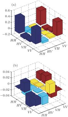
Experimentally, if the long-pass filters are used, then the measured nv, v = 1, … , 16 are: n1 = 6968, n2 = 558, n3 = 6250, n4 = 472, n5 = 3992, n6 = 3445, n7 = 2562, n8 = 4490, n9 = 3606, n10 = 6398, n11 = 3755, n12 = 2816, n13 = 4108, n14 = 3535, n15 = 3861, n16 = 6902. Therefore, the density matrix ρ of the entangled source is tomographically reconstructed as
We schematize various components of the real and imaginary parts of the density matrix ρ l in Fig. 4.
 | Fig. 4. Elements of the reconstructed density matrix ρ l: panel (a) is the image of the real part of the density matrix, and panel (b) is the image of the imaginary part of the density matrix. |
From the above reconstructed data, the purity of the entangled-source can be calculated as 
Alternatively, if the interference filters are used, then the relevant measured data read: n1 = 278, n2 = 8, n3 = 218, n4 = 2, n5 = 142, n6 = 125, n7 = 82, n8 = 133, n9 = 110, n10 = 278, n11 = 145, n12 = 87, n13 = 149, n14 = 137, n15 = 145, n16 = 309. As a consequence, the density matrix of the entangled-source becomes
with the elements are schematized is Fig. 5. Correspondingly, the relevant purity reads 
 | Fig. 5. Elements of the reconstructed density matrix ρ i: panel (a) is the image of the real part of the density matrix, and panel (b) is the image of the imaginary part of the density matrix. |
The above quantum state tomographic reconstructions show that the generated entangled-source is not exactly maximal entangled state. This indicates that the measurement settings used above for the primary tests of the BI are not the suitable settings, which should be reselected for the generated non-maximal entangled source. Therefore, the second step for the test should be optimizing the measurement settings for the specific entangled source.[26]
The probability of the coincidence count reads

for the arbitrary measurement setting

As a consequence, the value of the CHSH function S can be calculated by suing Eqs. (4), (12)– (13). With the Mathematica program[27] we can optimize the measurement settings to get the maximal value of the CHSH function. The relevant results are θ 1 = 109.98° , θ 2 = 35.22° , 


Finally, with the above optimized measurement settings, we perform the experimental test of the BI. The relevant data are listed in Table 2. With the measured data and from Eqs. (4) and (13), the values of the CHSH function can be obtained as: S = 2.450 ± 0.015 for the long-pass filters, and S = 2.772± 0.063 for the interference filters. Obviously, the degree of the violation of the BI has been enhanced, and the using of the interference filters increases the violation more significantly.
| Table 2. Experimental data of the measured coincidence counts for the measurement settings obtained by using the long-pass filters. |
| Table 3. Experimental data of the measured coincidence counts for the measurement settings obtained by using the interference filters. |
In summary, we discussd how to enhance the violation of the CHSH inequality by optimizing both the entangled source, via using the suitable filters, and the relevant measurement settings, and via the tomographic technique. Indeed, without the relevant optimizations, the primary tests, by assuming the generated entangled-source is the maximal entangled state, indicates the violation of the BI. However, the values of the violation degree, i.e., the CHSH function for the CHSH inequality, are relatively low: S = 2.390± 0.013 for using a pair of long-pass filters, and S = 2.735± 0.0617 for using the interference filters. Our works showed that these violations can be enhanced by further optimizing the measurement settings via the tomographic technique.
In fact, the tomographic reconstructions of the entangled-source showed that the polarization entangled-photon pairs generated by the pumping of our I-type BBO crystal are not the desirable maximal entangled states, although their purities are still very high. This implies that the measurement settings for the maximal entangled-state source are not the optimal ones for the tests of the BI. Therefore, based on the reconstructions of the entangled source, we optimized the measurement settings accordingly. With the reselected measurement settings, we found that the degrees of the violations of the BI are enhanced really; for the case of using the long-pass filters the value of CHSH function increased from 2.390± 0.013 to 2.450± 0.015, and for the case of using the interference filters the value of CHSH function increased from 2.735± 0.0617 to 2.772± 0.063.
In our experiments, two kinds of filters in the diaphragm are respectively used to increase the quality of the entangled-source. Our measured results showed that the purity by using the interference filters is better than that by using the long-pass filters, although the less coincident counts are obtained. This obstacle could be overcome by increasing the power of the pumping laser, at least in principle. It is emphasized that, the present work focused only on the increasing of the degree of the violation of the BI for approaching Cirelson’ s limit. Certainly, completeness testing of the BI needs to close the local and detection loopholes. This will be investigated in our future experiments.
After we finished this paper, we were aware of a stronger violation of the CHSH Bell inequality, i.e., S = 2.827 ± 0.017, has been demonstrated in a recent experiment.[28] We note that there are three differences between that work and the present one. Firstly, the laser used in that experiment is pulse-type, while in our experiment a continuous light source is used. Secondly, a BBO crystal is introduced to increase the efficiency of the entangled photon-pairs generated by pumping a BiBO crystal, however, in our experiment a BBO crystal to was simply used to produce the entangled photons. Finally, compared to our avalanche diode photon detectors the experiment reported in Ref. [28] used the transition-edge sensors (TESs) with higher coincidence counts. This is the main reason why the higher violation of Bell’ s inequality was obtained, and also provide a further approach to improve our experiment.
| 1 |
|
| 2 |
|
| 3 |
|
| 4 |
|
| 5 |
|
| 6 |
|
| 7 |
|
| 8 |
|
| 9 |
|
| 10 |
|
| 11 |
|
| 12 |
|
| 13 |
|
| 14 |
|
| 15 |
|
| 16 |
|
| 17 |
|
| 18 |
|
| 19 |
|
| 20 |
|
| 21 |
|
| 22 |
|
| 23 |
|
| 24 |
|
| 25 |
|
| 26 |
|
| 27 |
|
| 28 |
|