


Grazing bifurcation analysis of a relative rotation system with backlash non-smooth characteristic
[Liu Shuanga), b) , Wang Zhao-Long†a)  , Zhao Shuang-Shuang
a) , Li Hai-Bina), b) , Li Jian-Xiong]
, Zhao Shuang-Shuang|
|


†Corresponding author. E-mail: zlwang1988@163.com
*Project supported by the National Natural Science Foundation of China (Grant No. 61104040), the Natural Science Foundation of Hebei Province, China (Grant No. E2012203090), and the University Innovation Team of Hebei Province Leading Talent Cultivation Project, China (Grant No. LJRC013).
Grazing bifurcation of a relative rotation system with backlash non-smooth characteristic is studied along with the change of the external excitation in this paper. Considering the oil film, backlash, time-varying stiffness and time-varying error, the dynamical equation of a relative rotation system with a backlash non-smooth characteristic is deduced by applying the elastic hydrodynamic lubrication (EHL) and the Grubin theories. In the process of relative rotation, the occurrence of backlash will lead to the change of dynamic behaviors of the system, and the system will transform from the meshing state to the impact state. Thus, the zero-time discontinuous mapping (ZDM) and the Poincare mapping are deduced to analyze the local dynamic characteristics of the system before as well as after the moment that the backlash appears (i.e., the grazing state). Meanwhile, the grazing bifurcation mechanism is analyzed theoretically by applying the impact and Floquet theories. Numerical simulations are also given, which confirm the analytical results.
The relative rotation system, as a widespread energy transmission system in the project, has drawn much attention in recent years. Luo set up the theory of relativistic analytical mechanics of the rotational systems in 1996, [1– 3] which was applied to the research on the symmetry theory of dynamical systems.[4– 6] Various nonlinear factors are contained in the relative rotation system, which lead to the system to produce complex dynamic behaviors such as bifurcation and chaos. Bifurcation and chaos are important parts of the nonlinear scientific fields.[7– 10] They have achieved rapid development and extensive applications in the fields of secure communications[11– 13] and signal processing.[14– 16] At the same time, the Hopf bifurcation was analyzed on the basis of the relative rotation theory, and the nonlinear and nonlinear time-delayed feedback control techniques were proposed to control the bifurcation points and the stability of periodic solutions.[17– 19] The bifurcation response equation of the relative rotation system was deduced with the method of multiple scales, and the bifurcation and chaotic motions under combination resonance were investigated.[20, 21] The parameter stability and global bifurcations of a strong nonlinear system with parametric excitations and external excitations were investigated using the method of multiple scales.[22] The existence of both Hopf bifurcation and the topological horseshoe for a novel finance chaotic system was investigated.[23] The anti vibratory passive and active methods were applied to complex mechanical systems.[24] The nonlinear free vibrations of the electromechanical integrated toroidal drive system were investigated using the perturbation method.[25] However, all the systems studied in the above-mentioned literatures are smooth dynamical systems, in which the nonsmooth factors are neglected. In addition, some nonsmooth factors may lead to grazing bifurcation and induce the oscillatory instability.
Grazing bifurcation is a proprietary bifurcation in the nonsmooth dynamical system. The sliding and grazing bifurcations in periodically forced oscillators with dry friction were extensively investigated.[26– 28] A linear oscillator undergoing impacts with a secondary elastic support was studied, and both smooth and nonsmooth bifurcations were observed.[29] An impacting system was investigated, the results of which showed that the periodic windows in the locus of boundary crises were caused by grazing bifurcations intersecting the locus of boundary crises and that grazing bifurcations can affect the existence of the boundary saddle-point solutions.[30, 31] The existence and stability of the grazing periodic trajectory in a two-degree-of-freedom vibro-impact system were investigated.[32] The relationship between the saddle-node and grazing bifurcations in periodically-forced impact oscillators was investigated.[33] The complex oscillations caused by the occurrence of grazing bifurcations in a pressure relief valve were investigated.[34] A non-smooth model of a Jeffcott rotor was investigated. The study revealed a rich variety of dynamics, which included grazing-induced fold and period-doubling bifurcations.[35] However, the systems in the above-mentioned literatures are linear and impact systems, some of which were studied directly by numerical simulations. Up to now, there have only been a few researches about grazing bifurcations for nonlinear systems with nonsmooth properties from the perspective of theory and mechanism.
In this paper, considering the nonsmooth and nonlinear characteristics, the dynamical equation of a nonlinear relative rotation system with backlash non-smooth characteristic is deduced. The grazing bifurcation mechanism is theoretically analyzed. Numerical simulations are also given, which confirm the analytical results and show that the grazing bifurcation can lead to the chaotic motion. Moreover, the research in this paper provides a theoretical reference for the design and control of the transmission system in practical engineering.
The rest of the paper is organized as follows. The dynamic model of the nonsmooth relative rotation system with backlash is presented in Section 2. The grazing bifurcation mechanism is analyzed in Section 3. Numerical simulations are performed in Section 4, and some concluding remarks are provided in Section 5.
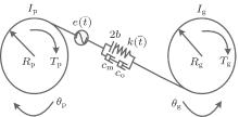
Considering the main drive system driven by an electrical motor, the transmissions between the motor and the load are gears. The motor and the drive gear are connected by a rigid shaft, so that they can be equivalent to a concentrated mass. A similar method can be applied to the load and the driven gear. Meanwhile, considering the influence of backlash, time-varying characteristics and oil film, the structure of the two-mass system is shown in Fig. 1.
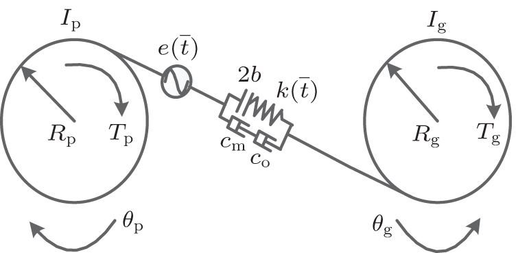 | Fig. 1. The dynamic model of nonsmooth relative rotation system with backlash. |
The parameters are as follows: Ip and Ig are the rotational inertias of the drive and driven gears, respectively, Rp and Rg are the base radiuses of the drive and driven gears, respectively, Tp and Tg are the input torque and the load torque, respectively, θ p and θ g are the vibratory angular displacements of the drive and driven gears, respectively, 2b is the total backlash, cm is the meshing damping coefficient, co is the oil film damping coefficient, k(t̄ ) is the time-varying stiffness, and e(t̄ ) is the static transmission error caused by manufacturing. Here,

where km is the mean mesh stiffness, kq is the variable amplitude of mesh stiffness, ω is the tooth mesh frequency, and

where ea is the variable amplitude of unload static error, ω is the tooth mesh frequency, and ϕ c is the initial phase.
The width of the backlash is determined by the linear displacement difference between the two gears, so the transmission error of the linear displacement is defined as

The backlash function is defined as

As shown in Fig. 1, the internal dynamic force can be expressed as

According to Newton’ s law, the dynamical equation of a relative rotation system with backlash nonsmooth characteristic under the oil film force can be expressed as

During the actual transmission process, the oil film damping is influenced by many factors. Meanwhile, when the backlash appears between the mating gear teeth, the oil will leak, so the oil film can be ignored. In this paper, the oil film damping is considered only when the mating gear teeth mesh with each other.
Under the conditions that the density and viscosity of the oil film are constant, the Reynolds equation is introduced, [36] which can be used to describe the distribution of pressure between the contact surfaces

where u = (up + ug)/2, h is the oil film thickness,
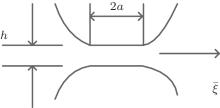
When the oil film thickness is constant in the contact area, the Grubin theory is introduced.[36] Therefore, the oil film thickness h is constant along the

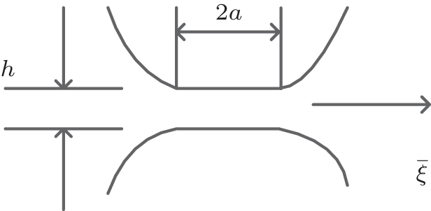 | Fig. 2. Grubin contact model. |
where α is the pressure– viscosity coefficient of oil, R is the equivalent radius, E′ is the equivalent elastic modulus, w is the load per unit length, a is the semi-width of the contact area, η 0 is the nominal oil film viscosity, and a = [8wR/(π E′ )]1/2. Then, equation (7) reduces to

By integrating Eq. (9) with the following boundary conditions:

p(

where l is the axial length of the contact area, and ∂ h/∂ t̄ is the squeezing velocity, i.e., ∂ h/∂ t̄ = q̇ . The negative sign indicates that the direction of the oil film force is opposite to the squeezing velocity direction of the oil film. If the squeezing velocity is positive, the oil film force is a damping force. Hence,

Let 


The dimensionless backlash function is

The dimensionless oil film force is

The dimensionless oil film damping is 

Let x = y − 1, and the system model can be rewritten as

Let x1 = x, x2 = ẋ , and x3 = Ω t, then, the state equation of the system can be expressed as

The state space is divided into three subspaces

where x = (x1, x2, x3)T, K(x) = x1,


Equation (18) is the dynamical state equation of the nonsmooth relative rotation system considering oil film damping, backlash, time-varying stiffness and time-varying error. The system is in a meshing state when x ∈ S1; the system is in an impact state when x ∈ S1 and x ∈ S2 simultaneously. Because of the existence of the backlash, the system will undergo different states. When the system makes the transition from the meshing state to the impact state, the solution trajectory of the system will cross the boundary K(x) = 0 and the motion state of the system will change, which may result in the state instability. Therefore, we will analyze the local behaviors of the system in the vicinity of the boundary.
In the process of transmission, on the moment that the backlash appears immediately, the solution trajectory of the system which is in the meshing state will hit the boundary tangentially without crossing it, which is defined as the grazing state. If a small perturbation caused by a system parameter is applied to the system, the backlash will appear between the meshing gears, which will result in the change of the dynamical behaviors of the system. The evolution of the grazing trajectory is shown in Fig. 3.
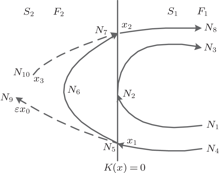 | Fig. 3. The schematic diagram of zero-time discontinuous mapping (ZDM). |
The solution trajectory N1 → N2 → N3 is the grazing trajectory. When influenced by a small perturbation caused by a system parameter, the grazing trajectory will cross the boundary and evolve into another trajectory N4 → N5 → N6 → N7 → N8. N4 → N5 and N7 → N8 are the segments of the trajectory controlled by the vector field F1 in the state space S1; N5 → N6 → N7 is the segment of the trajectory controlled by the vector field F2 in the state space S2; N5 → N9 and N10 → N7 are the segments of the virtual trajectories controlled by the vector field F1 when the boundary is ingnored. The zero-time discontinuous mapping (ZDM) is introduced to describe the influence of the vector field F2 on the dynamical behaviors of the system when the solution trajectory is crossing the boundary.
In order to compute the trajectory N4 → N5 → N6 → N7 → N8, the first segment (N4 → N5 → N9) can be computed using the vector field F1, even if it crosses the boundary. Then, the ZDM (i.e., N9 → N10) can be applied to take into account the fact that the system has crossed the boundary. Finally, the second segment (N10 → N7 → N8) can be computed using the vector field F1 again.
On the basis of this, choosing a fixed phase plane as the Poincare section, the Poincare mapping of the relative rotation system (18) with a backlash non-smooth characteristic under the oil film force is deduced by combining the ZDM. The Jacobian matrix of the Poincare mapping can be obtained when the ZDM is used as a special impact mapping. Then, the Floquet theory is applied to analyze the grazing bifurcation mechanism of the system.
When Pm > Pq, at x = (0, 0, 0)T, the system (18) satisfies the following grazing conditions:[37]


Thus, the grazing point is x* = (0, 0, 0)T, denoted by O. The ZDM is introduced to describe the influence of the vector field F2 on the dynamical behaviors of the system (18) when the solution trajectory is crossing the boundary.
The flows Φ i(x, t), i = 1, 2 (i.e., the solution trajectories of the system) which are generated by the vector fields Fi(i = 1, 2) of the system (18) can be defined as the quantities that satisfy

Now, because of the smoothness of the vector fields Fi(i = 1, 2), each of the system flows Φ i(x, t), i = 1, 2 can be expanded as a Taylor series about the grazing point as

Note that a shorthand notation has been used here for the higher-order derivative terms, for example

Using the expression in Eq. (23) and the fact that

We can obtain from Eq. (24) that

As shown in Fig. 3, the ZDM ε x0 → x3 is split into three pieces. Assuming that the time from ε x0 to x1 is − δ , the Taylor expansion of x1 about the grazing point becomes
At point x1, which is in the boundary, K(x1) = 0, so

By substituting the Taylor expansion of Eq. (26) into Eq. (27), the result is

where


where

Assuming that the time from x1 to x2 is Δ , following the same procedure as before, it is found that


Hence, it follows that

where


Assuming that the time from x2 to x3 is δ − Δ , in order to ensure that the total time is zero for the mapping ε x0 → x3, then,

The system (18) has a continuous form at the point of grazing discontinuity. At the grazing point, F1 = F2. This condition gives rise to a 3/2 singularity in the ZDM. Due to the continuous nature of the vector fields at the grazing point, O(ε 1/2) terms go to zero, and O(ε ) coefficients become x0. Further calculation of O(ε 3/2) terms yields the ZDM. Therefore, combining the actual formulas of F1 and F2 in system (18), the ZDM has a leading order term of the form

which is the ZDM denoted by G. Next, the Poincare mapping will be deduced to analyze the local dynamic characteristics in the vicinity of the grazing point.
In order to obtain the Poincare mapping in the vicinity of the grazing point, a fixed phase plane is chosen as the Poincare section

where T = 2π /Ω .
When the solution trajectory of the system does not cross the boundary, the system is controlled by the vector field F1 and the Poincare mapping is a smooth mapping

The Psmooth is defined as

When the solution trajectory of the system crosses the boundary, the system is controlled by the vector field F1 and the vector field F2, and the ZDM is introduced to describe the influence of the vector field F2 and the boundary on the dynamical behaviors of the system, so the Poincare mapping is a nonsmooth composite mapping as

The Pnonsmooth is divided into three local mappings


Then, the Poincare mapping is

where P3 ○ P2 ○ P1 represents P3(P2(P1)), i.e., x0+ T = P(x0) = P3(P2(P1(x0))).
The Poincare mapping can describe the change of the dynamical behaviors of the system in the vicinity of the grazing point.
The change of the largest eigenvalue of the Jacobian matrix in the Poincare mapping can be used to analyze the change of the dynamical behaviors of system (18).
The ZDM which is a discrete mapping, just like the impact mapping, is regarded as a special impact mapping in this paper. Therefore, the Jacobian matrix of the Poincare mapping can be obtained by applying the impact theory.
When the solution trajectory of the system does not cross the boundary, the Jacobian matrix of the Poincare mapping which is a smooth mapping can be obtained by integrating Eqs. (43) and (44) from t0 to t0 + T

where I3 is a 3 × 3 unit matrix, J is the Jacobian matrix at a certain moment, and F1 is the vector field of system (18)

where x0 is the initial value.
The Jacobian matrix of the Poincare mapping is

When the solution trajectory of the system crosses the boundary, the Jacobian matrix of the Poincare mapping which is a nonsmooth composite mapping can be expressed as

Here, P1 and P3 are both smooth mappings. Thus, DP1 can be obtained by integrating Eqs. (43) and (44) from t0 to t* ; DP3 can be obtained by integrating Eqs. (43) and (44) from t* to t0 + T − t* .
According to the impact theory, DP2 is given by[34]

where Gx = ∂ G/∂ x, Kx = ∂ K/∂ x.
In conclusion, the Jacobian matrix of the Poincare mapping in the vicinity of the grazing point can be expressed as

The change of the largest eigenvalue of the Jacobian matrix (47) can be used to analyze the grazing bifurcation mechanism of the system (18). The results are obtained according to the above analysis and the Floquet theory:
Theorem 1 If all the eigenvalues of the matrix DP in Eq. (47) are within the unit circle, the system is stable. Otherwise, the system will lose its stability. With the decrease of Pm, the grazing bifurcation will occur when the largest eigenvalue jumps out of the unit circle.
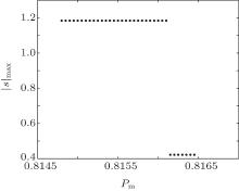
The external excitation influenced by the torque ripple or exterior factors is chosen as the bifurcation parameter to study the system. The system parameters are chosen as ς = 0.04, σ = 0.1, Pq = 0.81, Ω = 0.1, η = 1.2, c = 0.1207 × 10− 3. The change of the modulus of the largest eigenvalue of the Jacobian matrix (47) in the local area 0.8148 ≤ Pm ≤ 0.8165 is shown in Fig. 4.
 | Fig. 4. The change diagram of the modulus of the largest eigenvalue. |
As shown in Fig. 4, when Pm ≥ 0.8162, the modulus of the largest eigenvalue is less than 1, which means that all the eigenvalues are within the unit circle, so the system is stable; when Pm < 0.8162, the modulus of the largest eigenvalue is greater than 1, which means that the largest eigenvalue jumps out of the unit circle, so the system becomes instable. The grazing bifurcation point is Pm = 0.8162.
Next, the nonsmooth relative rotation system (18) will be analyzed to prove the validity of the conclusion. The bifurcation diagram of the system (18) is shown in Fig. 5.
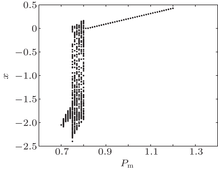 | Fig. 5. The bifurcation diagram of system (18). |
It can be seen from Fig. 5 that, with the decrease of Pm, the system in the single periodic stable motion undergoes the grazing motion and it later becomes chaotic motion because of the grazing bifurcation. When Pm > 0.82, the system is in the single periodic stable motion. Meanwhile, the system is in the meshing state; when Pm < 0.82, the system is in the chaotic motion. Meanwhile, the system is in the impact state. The grazing bifurcation point is Pm = 0.82. The ZDM is the approximate calculation of the system, so there are some errors.
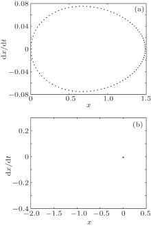
The phase diagrams and the Poincare sections with different values of Pm are shown in Figs. 6– 8. As depicted in Figs. 6(a) and 6(b), when Pm = 0.84, the system which has not undergone the grazing state is in the single periodic stable motion. Meanwhile, the system is in the meshing state. As shown in Figs. 7(a) and 7(b), when Pm = 0.82, the system stays in the grazing state exactly, and its dynamical behavior has not changed, and the system is in the critical meshing state. When Pm = 0.80, the system enters chaotic motion after the grazing state, and the system is in the impact state. The ruleless state shown in Fig. 8(a) and the obvious fractal structures shown in Fig. 8(b) can prove the existence of the chaotic motion.
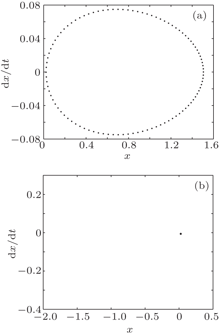 | Fig. 6. The phase diagram and the Poincare section of Pm = 0.84. (a) The phase diagram. (b) The Poincare section. |
 | Fig. 7. The phase diagram and the Poincare section of Pm = 0.82. (a) The phase diagram. (b) The Poincare section. |
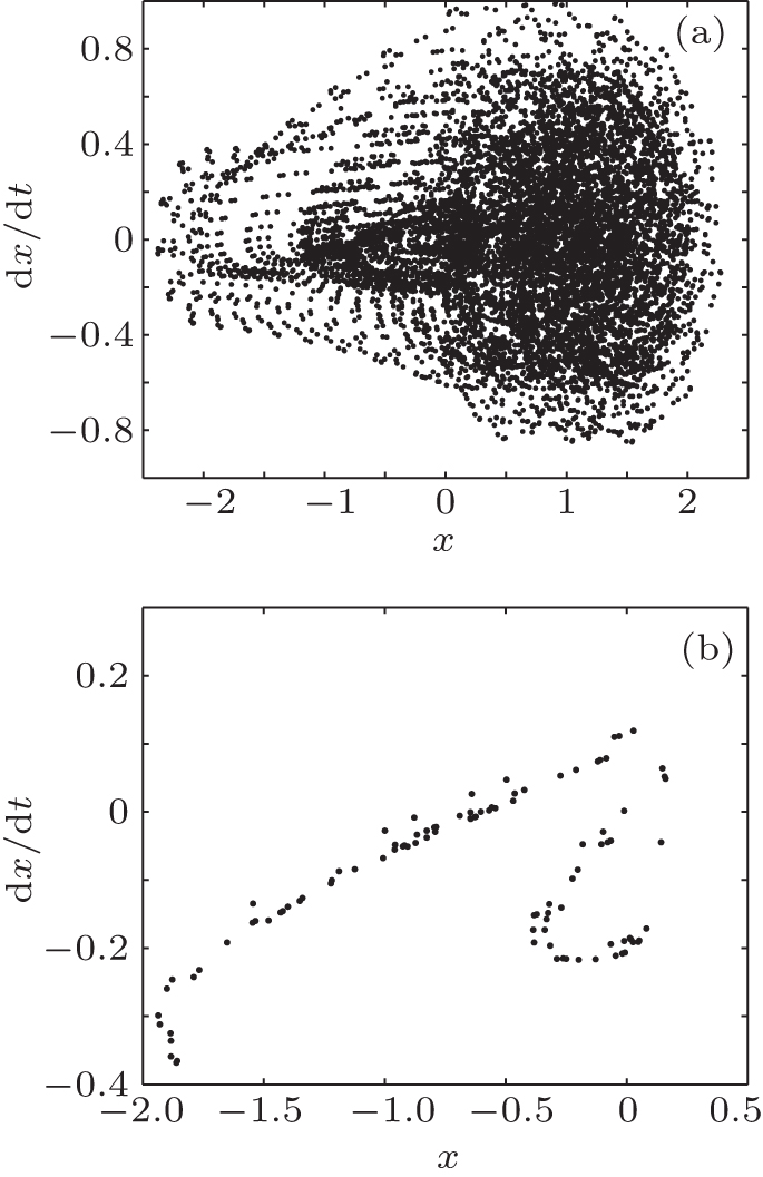 | Fig. 8. The phase diagram and the Poincare section of Pm = 0.80. (a) The phase diagram. (b) The Poincare section. |
In this paper, considering the oil film, backlash, time-varying stiffness, and time-varying error, the dynamical equation of a relative rotation system with the backlash nonsmooth characteristic is deduced according to Newton’ s law. The grazing bifurcation mechanism of the system is analyzed as the external excitation changes. The research shows that with the decrease of the external excitation, the system transforms from the meshing state to the impact state. During this period, the grazing bifurcation occurs so that the dynamical behaviors of the system change from the single periodic stable motion to the chaos motion. Increasing the external excitation is propitious to suppressing the chaotic behaviors caused by the grazing bifurcation. These results have an important theoretical significance on reducing the vibration of the relative rotation systems with backlash. In addition, the research in our paper provides a reference for the further study of complex nonsmooth dynamic behaviors of large rotary machinery.
| 1 |
|
| 2 |
|
| 3 |
|
| 4 |
|
| 5 |
|
| 6 |
|
| 7 |
|
| 8 |
|
| 9 |
|
| 10 |
|
| 11 |
|
| 12 |
|
| 13 |
|
| 14 |
|
| 15 |
|
| 16 |
|
| 17 |
|
| 18 |
|
| 19 |
|
| 20 |
|
| 21 |
|
| 22 |
|
| 23 |
|
| 24 |
|
| 25 |
|
| 26 |
|
| 27 |
|
| 28 |
|
| 29 |
|
| 30 |
|
| 31 |
|
| 32 |
|
| 33 |
|
| 34 |
|
| 35 |
|
| 36 |
|
| 37 |
|