Rotational stretched exponential relaxation in random trap–barrier model
[Aydiner Ekrem† ]
]
]
|
|


†Corresponding author. E-mail: ekrem.aydiner@istanbul.edu.tr
*Project supported by Istanbul University (Grant Nos. 28432 and 45662).
The relaxation behavior of complex-disordered systems, such as spin glasses, polymers, colloidal suspensions, structural glasses,and granular media, has not been clarified. Theoretical studies show that relaxation in these systems has a topological origin. In this paper, we focus on the rotational stretched exponential relaxation behavior in complex-disordered systems and introduce a simple phase space model to understand the mechanism of the non-exponential relaxation of these systems. By employing the Monte Carlo simulation method to the model, we obtain the rotational relaxation function as a function of temperature. We show that the relaxation function has a stretched exponential form under the critical temperature while it obeys the Debye law above the critical temperature.
Complex systems generally show strongly non-exponential dynamics, which are defined by the stretched exponential relaxation (SER) in the form

where τ is a macroscopic relaxation time, and α denotes the empirical exponent, which has a value between 0 and 1 depending on the physical properties of the system. The upper limit of α = 1 corresponds to a simple exponential decay, [1] while lower values of α are indicative of a more complicated nonexponential relaxation process, giving rise to a fat tail. In 1854, Kohlrausch used this expression to parameterize polarization decay data in Leiden jars.[2] In 1970, this form was used by Williams and Watts to explain the relaxation of dielectric systems.[3] Because of historical reasons, the SER is also called as Kohlrausch– William– Watts relaxation. It has been shown that the SER gives an excellent representation of experimental and numerical relaxation data in a huge variety of complex systems, including polymers, colloidal suspensions, structural glasses, [4– 7] spin glasses, [8– 10] granular media, [11, 12] and many more. However, the physical mechanism behind the SER in these systems has not been clarified. Hence, the SER behavior of the complex systems is still widely regarded as one of the most challenging unsolved problems in condensed matter physics.[13, 14] The common properties of these systems are the non-crystalline structure, non-equilibrium dynamics, and non-ergodic thermodynamics. Slow dynamics can occur depending on one or all of these physical ingredients of the systems. The SER behavior is very complex in spin glass systems because they include the three physical ingredients mentioned above. Here, we focus on rotational SER dynamics in Ising spin glass systems and introduce a simple model.
Many theoretical models have been proposed to explain the SER behavior of complex-disordered systems.[13] In addition, there are a number of other theories that show SER behavior, such as spin models, [15] diffusion-trap models, [13, 16– 21] hierarchical models, [22] and the model of random walkers on dilute hypercubes of high dimensions.[23– 29] Theoretical studies suggest that the stretching exponent has an inherently topological origin.[4, 9, 23– 29] Therefore, the relaxation of complex-disordered systems can be modeled by the diffusion-trap and percolation models. These models suggest that a large number of meta-stable states with very high degeneracy exist in the phase space of the systems, which are separated from each other by huge barriers when the systems, for example spin glasses, are cooled to low temperature under an external field[30– 33] and the systems freeze into one of the many ground states. So multi-valley landscape of the free energy enforces the systems to non-exponential dynamics. According to the topological models, in the phase space, each minimum in the ground sates corresponds to one of the eigen-states of the system. The ensemble of all possible configurations in the available phase space at temperature T can be considered as the set of eigen-states of the system at the micro canonical level. The number of eigen-states (i.e., the available phase space) changes with temperature. At high temperature, the system has a large number of microstates (i.e., available eigen-states). However, the number of available eigen-states decreases with decreasing T. According to this scenario, when the system moves from one of eigen-state to another, the system begins relaxing to the equilibrium state. However, the multi-valley landscape of the free energy enforces the system to glassy dynamics. Thus, the relaxation of the system fits to SER near the glassy or frozen temperature Tc due to the large number of available states thermally permitted. Campbell et al. suggested that the morphology of phase space of a complex-disordered system can be represented by a d-dimensional percolated hypercube, where each energy eigen-state of the system corresponds to a vertex of the hypercube. They showed that relaxation in the percolated hypercube fits to the SER.[23– 29]
In this study, to discuss the rotational stretched exponential relaxation in complex-disordered systems, we suppose that the random trap-barrier (RTB) model, which has not been used yet to model the stretched exponential relaxation in complex systems, may create a more realistic d-dimensional phase space morphology for the complex disordered systems than other models. For simplicity, we only focus on d = 3 case (i.e., a simple spherical surface). The organization of this paper is as follows. In Section 2, we introduce the RTB model. In Section 3, we define a rotational relaxation function based on the analytical method in Ref. [34] to use in the simulation. In Section 4, we give details of the simulation and results. Finally, a conclusion is given in Section 5.
The RTB model was introduced by Limoge and Boequet to explain an Arrhenian temperature dependence of the diffusion coefficient in amorphous substances.[35] The simple one-dimensional schematic representation of the RTB model was given in Ref. [35], which is the combination of random trap (RT) and random barrier (RB) models. Now we extend the one-dimensional RTB model to spherical geometry and investigate the rotational relaxation considering a 3-dimensional hypercube correspond to a simple spherical lattice network. We assume that the vertices and bonds of the spherical lattice network are consist of random traps and random barriers.
In this model, the trap energy and the barrier energy are restricted to E ≤ 0 and E ≥ 0, respectively. E(θ , ϕ ) is the random trap energy of site (θ , ϕ ), counted negative from a common origin; and E(θ , ϕ ; θ ′ , ϕ ′ ) is the random barrier energy between sites (θ , ϕ ) and (θ ′ , ϕ ′ ). To construct the spherical RTB lattice network for simulation, the trap energies E(θ , ϕ ) and barrier energies E(θ , ϕ ; θ ′ , ϕ ′ ) are randomly distributed between − 1 and 1. The traps and barriers create a static phase space structure and their configurations remain unchanged for the duration of the simulation.
The transition or jumping probability of a particle from vertex of sphere-like lattice (θ , ϕ ) to (θ ′ , ϕ ′ ) is given by

Similarly, the transition probability from lattice vertex (θ ′ , ϕ ′ ) to (θ , ϕ ) is given by

The detailed balance condition is satisfied between two neighbor vertices on the surface of the sphere-like lattice RTB network and is given by

and the thermal occupation factor π (θ , ϕ ) is defined by
The occupation factors are proportional to the thermal equilibrium occupation probabilities of the sites. The curly brackets in Eq. (5) designate the average over the disordered site energies for finite segments

The numerator contains only barrier energies, while the site energies only appear in the denominator, which can be evaluated directly.
According to the rotational relaxation scenario, a spin or dipole moment can be considered as a unit vector which is initially (at t = 0) directed to θ = 0 and randomly rotates to θ or ϕ direction with time t. The rotational relaxation in this relaxation scenario can be defined in terms of time autocorrelation function as
where Ylm(θ , ϕ ) is the spherical harmonics and ⟨ · · · ⟩ indicates the expectation value. The expectation value of 

where (Ω 0, t0) ≡ (θ , ϕ ; θ ′ , ϕ ′ , t0), (Ω , t) ≡ (θ , ϕ ; θ ′ , ϕ ′ , t), and P(Ω 0, t0) and P(Ω , t) in are the conditional probabilities of jumping from one vertex to another on the spherical-like lattice network. To calculate the expectation value in Eq. (8) the conditional probability P(Ω , t) needs to be known.
Fortunately, such a rotational relaxation process can be mapped to diffusion on a sphere. Therefore, the rotational relaxation of a spin or dipole moment can be modeled in terms of diffusion. For ordered systems, Debye showed that P(Ω , t) can be the solution of a diffusion equation in the spherical coordinates. The comprehensive solution can be found in Ref. [1]. For l = 1 and m = 0, relation (7) reduces simply to q(t) = ⟨ cosθ (t)⟩ , hence the rotational relaxation function is given by

where the probability distribution function satisfies P(θ , t) = δ (θ ) for t = 0. The analytical solution of rotational relaxation for ordered systems gives the exponential relaxation

However, the presence of geometrical or energetical restrictions on the surface or lattice diffusion leads to

This equation is known as the fractional diffusion equation. In Eq. (11), P(θ , ϕ , t) is the probability function of the particles on the spherical surface, 

which satisfies fractional diffusion equation (11). If we put Eq. (12) into Eq. (9), then

The rotational relaxation function (13) is valid for an arbitrary number l, however for a simple sphere, we take l = 1. An interesting property of relaxation function (13) due to the behavior of the Mittag– Leffler functions lies in that it interpolates to the initial SER behavior

Solution (14) causes to Eq. (1) for 0 < α < 1 and the Debye relaxation in Eq. (10) can be recovered at α = 1.
It can be seen from Eqs. (10) and (14) that the analytical solution of rotational relaxation can be obtained using mathematical models.[1, 34] However, these models do not depend on the microscopic details of the physical systems because the analytical models are hypothetical. In this work, we will obtain the rotational relaxation function for the RTB model with the help of MC simulation. In order to obtain rotational relaxation function q(t), firstly, we will compute the probability function P(θ , ϕ , t) in Eq. (12) for the model mentioned above from simulation at fixed temperature and compute 

where Δ θ is the angle belt on the sphere surface, and P(Δ θ , t) is the finding probability of the particles on the belt Δ θ at any time t.
In our Monte Carlo simulation scenario, non-interacting N particles at t = 0 locate at θ = 0 with probability P(θ = 0, t = 0) = δ (θ = 0). The probability satisfies the condition ∑ δ (θ = 0) = 1 at t = 0. All particles start to diffuse on the discrete RTB sphere for t > 0. Particles activated by temperature independently try to move one-step randomly from (θ , ϕ ) to (θ ′ , ϕ ′ ) in the Monte Carlo metropolis algorithm. Each particle at every time step can jump with a probability or wait. In both cases, the time is increased by one unit. All of the particles diffuse on the sphere in a similar way until the system reaches an equilibrium. It can be assumed that the system has reached equilibrium when the finding probability density is equally distributed on the sphere sites (θ , ϕ ) or between all angle belts Δ θ .
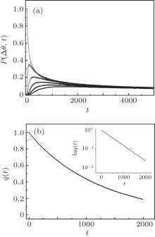
Firstly, we simulate particles over the discrete sphere which have no trap on vertices or barrier between vertices using non-interacting N = 100 particles. The time dependence of the normalized probability distribution function P(Δ θ , t) of the particles for different Δ θ angle intervals is plotted in Fig. 1(a). As can be seen from Fig. 1(a), the probability for each interval reaches saturation with time. When the system reaches saturation, the particles are distributed homogenously on the sphere surface. Physically, the saturation denotes that the system reaches to the equilibrium. On the other hand, to check the time dependent behavior of the rotational relaxation function for an ordered phase space, using data in Fig. 1(a), we plot q(t) Fig. 1(b). As can be seen from the inset in Fig. 1(b), the rotational relaxation function exponentially decays with time as exp(− t/τ ). This result obtained from the Monte Carlo simulation is compatible with numerical and theoretical results, [1] which confirms that our theoretical approach and simulation technique is true.
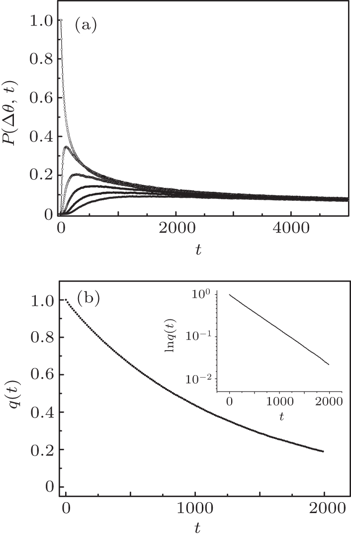 | Fig. 1. (a) The time dependence of the normalized probability distribution function P(Δ θ , t) for different angles Δ θ = 5, 10, 15, 20, 25, 30. (b) The time dependence of the rotational relaxation function for a sphere surface. The inset shows the exponential decay of q(t). |
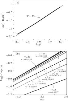
To obtain rotational relaxation function q(t) for the discrete RTB sphere, the simulation is carried out according to the scenario mentioned above. The simulation results of the RTB model are given as follows. In the RTM model simulation, to obtain good statistical averages, the MC simulations have been repeated over m = 500 different static discrete RTB sphere configurations and the numbers of particles for each independent simulation has been set as N = 1000. By using the RTB simulation data, the log(− ln q(t)) versus log (t) plot of q(t) for fixed temperature T = 50 is shown in Fig. 2(a). As can be seen in Fig. 2(a), the simulation data well fit to the SER; i.e., the stretched exponential function

where α is the SER decay exponent, τ is the macroscopic relaxation time, and q0 is the normalized constant. The SER relaxation exponent has a value in interval 0 < α < 1. Exponent α in static phase space configuration models is a measure of the geometric or energetic restrictions such as traps and barriers. It is suggested that the driving force in the static model is temperature. Hence, α changes depending on the temperature. To investigate the temperature dependence of α , we plot the rotational relaxation function q(t) for different temperatures in log(− lnq(t)) ∼ log(t) (Fig. 2(b)). As can be clearly seen from the figure, when the temperature decreases, the relaxation decays more slowly with time. The relaxation function clearly has an SER behavior for different temperatures. The slow decay of the relaxation function shows that the number of available microstates (i.e., eigen-states) effectively decreases when the temperature decreases. Indeed, the transition probability of the particles decreases at low temperature; hence, the particles do not move, and a viscous medium emerges due to the presence of the static traps and barriers. That is, when the temperature is lowered, the entropy drops and the number of thermally permitted vertices decreases, which means that diffusion in the system decreases. However, at relatively high temperatures, the diffusion effectively increases, the entropy of the system is high, and the number of the available microstates effectively increases.[17– 27, 29]
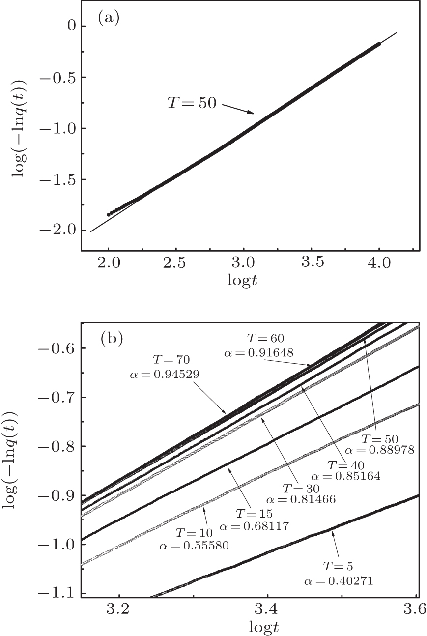 | Fig. 2. (a) The log(− ln q(t)) versus logt plot of the rotational relaxation function q(t) for temperature T = 50. The solid line on the curve is a fit line, which shows that the time dependence of simulation data can be represented by the stretched exponential relaxation function for the spherical RTB model. (b) The log(− ln q(t)) versus log(t) plot of the rotational relaxation function q(t) for different temperatures. |
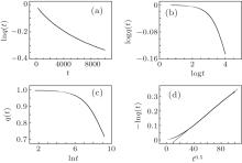
Figures 2(a) and 2(b) clearly show that the RTB model leads to SER rotational relaxation. However, to see whether or not our simulation data obey the SER form, we plot the data for T = 10 in Fig. 3 in the forms of (a) ln q(t) versus t, (b) log q(t) versus logt, (c) q(t) versus lnt, and (d) − ln q(t) versus t0.5. As can be seen in Figs. 3(a)– 3(c), there are no exponential, power, or logarithmic dependencies in our simulation data. It is clear that the data are compatible with SER behavior, particularly for long times. Here we believe that figure 3(d) is a powerful tool to check whether or not the data obey the SER. The figures confirm that the obtained simulation results for the RTB model are compatible with the experimental observations[8, 13] and the theoretical predictions.
 | Fig. 3. Numerical data for T = 10 are plotted: (a) ln q(t) versus t, (b) log q(t) versus logt, (c) q(t) versus lnt, (d) − ln q(t) versus t0.5. |
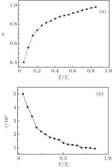
To determine the transition temperature at which the behavior of the system goes from exponential to stretched exponential relaxation, we analyze the temperature dependence of the relaxation exponent α . The temperature dependence of exponent α is shown in Fig. 4(a). As can be seen in Fig. 4(a), the relaxation exponent α increases up to one when the temperature is increased. The stretched exponential relaxation for the RTB model occurs nearly under T/Tc = 1, where Tc is the temperature at which the transition from ordered to complex or disordered phase occurs. However, at low temperatures, the exponent α slowly decreases to a critical value nearly α ≈ 0.3. On the other hand, it can be expected that the relaxation time τ increases when the temperature is decreased (Fig. 4(b)). Therefore, we can generalize these results. For T/Tc < 1, the relaxation exponent takes value α < 1, this means that the stretched exponential relaxation appears under this condition and q(t) ∼ exp [− (tα /τ α )]. For T/Tc > 1, the relaxation exponent takes α = 1, which is known as the Debye type relaxation q(t) ∼ exp [− (t/τ )]. Hence, the transition behavior can be presented with a scaling function, which depends on temperature

where for T/Tc < 1, the scaling function is given by f(T/Tc) = 1, and for T/Tc > 1, the scaling function is given by f(T/Tc) = exp [− (t1− α /τ α )].
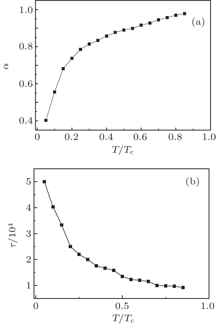 | Fig. 4. (a) The temperature dependence of the stretched exponential relaxation exponent α . (b) The temperature dependence of the macroscopic time τ . |
In the present study, we have obtained the rotational relaxation function for the sphere using a simple phase space model. We have also discussed the stretched exponential relaxation mechanism in complex-disordered systems. In addition, we investigate the temperature dependence of the stretched exponential rotational relaxation. Our Monte Carlo simulation results clearly show that the rotational relaxation function for different temperature decays stretched exponentially with time when T/Tc < 1. Here we must note that the SER may occur above the critical temperature in some of the complex disordered systems. For example, it has been reported that the SER occurs in spin glass systems above the frozen temperature. Relaxation in Ising spin glasses has been modeled by Campbell by using a percolated hypercube.[23] In percolation models, the threshold value pc corresponds to the critical temperature for glassy behavior of the system and relaxation does not occur below pc.
As can be seen from the previous studies, the SER is a ubiquitous feature of complex disordered systems which can be derived from trap diffusion and percolation models. Although the RTB is a very simple model, it may represent the phase space morphology of complex disordered systems rather than other phase space models, such as trapping and percolating models. Therefore, it can be used to model the rotational or translational relaxation in complex and disordered systems. Finally, we state that in the present study, the RTB model is simple but more pedagogical, which produces the SER behavior. On the other hand, the RTB can be easily extended to the higher dimensional hypercube.
| 1 |
|
| 2 |
|
| 3 |
|
| 4 |
|
| 5 |
|
| 6 |
|
| 7 |
|
| 8 |
|
| 9 |
|
| 10 |
|
| 11 |
|
| 12 |
|
| 13 |
|
| 14 |
|
| 15 |
|
| 16 |
|
| 17 |
|
| 18 |
|
| 19 |
|
| 20 |
|
| 21 |
|
| 22 |
|
| 23 |
|
| 24 |
|
| 25 |
|
| 26 |
|
| 27 |
|
| 28 |
|
| 29 |
|
| 30 |
|
| 31 |
|
| 32 |
|
| 33 |
|
| 34 |
|
| 35 |
|