
In-situ measurement of magnetic field gradient in a magnetic shield by a spin-exchange relaxation-free magnetometer*
[Fang Jian-Chenga) , Wang Taoa)†  , Zhang Hong
b) , Li Yanga) , Cai Hong-Weia) ]
, Zhang Hong|
|


†Corresponding author. E-mail: wangtao@buaa.edu.cn
*Project supported by the National Natural Science Foundation of China (Grant Nos. 61227902, 61374210, and 61121003).
A method of measuring in-situ magnetic field gradient is proposed in this paper. The magnetic shield is widely used in the atomic magnetometer. However, there is magnetic field gradient in the magnetic shield, which would lead to additional gradient broadening. It is impossible to use an ex-situ magnetometer to measure magnetic field gradient in the region of a cell, whose length of side is several centimeters. The method demonstrated in this paper can realize the in-situ measurement of the magnetic field gradient inside the cell, which is significant for the spin relaxation study. The magnetic field gradients along the longitudinal axis of the magnetic shield are measured by a spin-exchange relaxation-free (SERF) magnetometer by adding a magnetic field modulation in the probe beam’s direction. The transmissivity of the cell for the probe beam is always inhomogeneous along the pump beam direction, and the method proposed in this paper is independent of the intensity of the probe beam, which means that the method is independent of the cell’s transmissivity. This feature makes the method more practical experimentally. Moreover, the AC-Stark shift can seriously degrade and affect the precision of the magnetic field gradient measurement. The AC-Stark shift is suppressed by locking the pump beam to the resonance of potassium’s D1 line. Furthermore, the residual magnetic fields are measured with σ+- and σ–-polarized pump beams, which can further suppress the effect of the AC-Stark shift. The method of measuring in-situ magnetic field gradient has achieved a magnetic field gradient precision of better than 30 pT/mm.
Atomic magnetometers are widely studied and have developed rapidly in recent years.[1– 6] One of the most sensitive atomic magnetometers is the spin-exchange relaxation-free (SERF) atomic magnetometer, whose theoretical sensitivity can reach attotesla-level, [7] which can be used in biomagnetism, electric dipole moment (EDM) measurement, and ultrahigh sensitive inertial measurement.[8– 10] Furthermore, the SERF magnetometer has realized the highest sensitivity at low frequency.[11] The condition of a low residual magnetic field is essential in keeping the atoms in the SERF regime, which can result in the spin-exchange rate far exceeding the Lamor procession frequency.[12] Therefore, a passive magnetic shield and active magnetic compensation methods are always used in the atomic magnetometer to shield the earth’ s magnetic field.[13, 14] However, there is a small magnetic field gradient in the shield, which would increase the relaxation rate of the alkali atoms.[15] Therefore, precisely measuring the magnetic field gradient is vital to the spin relaxation study. The residual magnetic field along the longitudinal direction of the magnetic shield is always much larger than along the transverse direction due to the unequal shielding factor.[16] We are mainly concerned with the magnetic field gradient in the longitudinal direction in experiment. The magnetic field gradient in the magnetic shield is mainly comprised of two parts: one is the residual magnetic field gradient in the magnetic shield and the gradient effect introduced by the coils; the other is caused by the AC-Stark effect, which is also called light shift, and can be treated as fictitious magnetic field.[7] This is particularly true if the power of the pump beam cannot fully polarize the alkali atoms. The pump beam can then propagate through the cell with a uniform intensity, because the light shift is proportional to the intensity of the pump beam, which has a gradient along the direction of the pump beam. This light shift can seriously degrade and affect the precision of the magnetic field gradient measurement.
It is difficult to measure magnetic field gradient in the region of a cell, whose length of side is several centimeters. The size of the magnetometer’ s sensor needs to be less than several centimeters, and the spatial resolution of the magnetometer should be of the order of a few millimeters. The SERF magnetometer has realized a 2-mm spatial resolution, which was determined by the diffusion constant.[17] Moreover, the high spatial resolution makes the SERF magnetometer suitable for working in the structure of magnetometer arrays.[17] Furthermore, the SERF magnetometer is an ideal vector magnetometer, which can work as a three-axis magnetometer and realize in-situ magnetic field measurements.[18]
In this paper, we propose a method to realize the in-situ measurement of the magnetic field gradient in a cell, which is placed into a magnetic shield. The alkali atoms in the cell are kept in SERF regime by magnetic field shielding and compensation. Meanwhile, the structure of the probe beam optical system is designed to be suitable for detecting the magnetic field along the pump beam direction (the pump beam propagates along the longitudinal axis of the magnetic shield). The magnetic field is measured in steps of 2 mm along the pump beam, which can be used to calculate the magnetic field gradient. To measure the residual magnetic field along the pump beam direction, which is usually accomplished with the first harmonic signal of the lock-in amplifier, it is important to keep the transmissivity of the cell uniform with respect to the probe beam along the pump beam direction. However, this requires very exquisite manufacturing technology of the cell. Furthermore, the adhesion of the alkali atoms to the cell’ s wall can hardly be solved. The method of measuring the magnetic field gradient, proposed in this paper, is independent of the cell transmissivity, which is a significant development in the actual experiment. This method enables the measurement of the magnetic field gradient in the magnetic field to be performed more precisely and easily. The light shift and its gradient cannot be easily distinguished from the magnetic field, which can affect the precision of the magnetic field gradient measurement. To evaluate the magnetic field gradient caused by the residual magnetic field, the pump beam is locked to the D1 line of the potassium, which can greatly reduce the AC-Stark shift. Additionally, the light shift is further reduced by magnetic field measurement with σ + - and σ – -polarized pump beams.
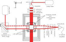
Due to the suppression of the spin-exchange relaxation, the SERF magnetometer is ultra-highly sensitive to the magnetic field.[12] The SERF magnetometer is a vector magnetometer, whose most sensitive direction is perpendicular to the probe beam and the pump beam. However, the SERF magnetometer can realize the three-direction magnetic field measurement by some modulation methods.[19, 20] As shown in Fig. 1, the probe beam propagates along the x direction, the pump beam propagates along the z direction, and the y direction is perpendicular to the probe beam and the pump beam. The spin evolution of the SERF magnetometer can be well described by the Bloch equation, [21]

where P is the electron spin polarization, q is the slowing-down factor, γ e is the gyromagnetic ratio of the electron, B is the residual magnetic field, the BLS is the light shift in the z direction, ẑ is the unit vector of the z direction, Rtot is the total spin relaxation rate, and ROP is the pumping rate of the pump beam, which can be considered as
 | Fig. 1. Experimental apparatus. A cubic cell is placed into the center of the magnetic shield and the compensation coils. A circularly polarized pump beam pumps the atoms along the z direction. A linearly polarized probe beam propagates along the x direction. The mirror mounted on the linear stage allows the probe beam to translate along the z direction. |
where re is the radius of the electron, c is the speed of light, fD1 is the oscillator strength of the D1 transition, Φ is the total flux of photons incident on the atom in units of number of photons per area per time, s is the photon spin vector, which ranges from − 1 to 1, ν p is the frequency of the pump beam, and ν D1 is the resonance frequency of the D1 transition, P is the power of the pump beam, A is the area of the pump beam, and h is the Planck constant.
The quasi-static solution of Eq. (1) can be considered as

where Px is the spin polarization in the x direction, P0 is the electron polarization, Bx, By, and Bz are the residual magnetic fields in the x, y, and z directions, respectively and


The light shift can be treated as a fictitious magnetic field, which can be considered as[7]

To keep the atoms in the SERF regime, the magnetic fields in three directions are well compensated. Moreover, the light shift cannot be easily distinguished with the magnetic field. Therefore, in order to precisely measure the residual magnetic field gradient in the magnetic shield, the light shift needs to be greatly reduced. According to Eq. (6), the light shift can be suppressed by locking the pump beam to the resonance of the potassium’ s D1 line. Then, an oscillating magnetic field modulation is used in the x direction to make the SERF magnetometer sensitive to the magnetic field in the z direction,

After the compensation of the magnetic fields, the residual magnetic fields in three directions and the light shift are relatively small, i.e., 

where Bg is the residual magnetic field after the magnetic field compensation, which is caused by the non-uniform magnetic field along the z direction.
The signal of the SERF magnetometer is acquired by measuring the optical rotation of the probe beam. Furthermore, the optical rotation can be considered as[7]

where nK is the vapor density of the potassium, l is the propagation length of the probe beam through the cell, fD2 is the oscillator strength of the potassium’ s D2 line, which is approximately 2/3, V is the Voigt profile, ν m is the frequency of the probe beam, and ν D2 is the resonance frequency of the potassium’ s D2 line.
The signal of the probe beam is detected by a photodiode, and the signal from the photodiode is demodulated by a lock-in amplifier. The modulated intensity on the photodiode can be considered as[22]

where I is the intensity of the probe beam, which is detected by the photodiode; I0 is the initial intensity of the probe beam; α is the retardation angle of the photoelastic modulator (PEM); ω is the modulation frequency of the PEM. From Eq. (10), we can find that the first harmonic ω is proportional to the optical rotation θ , and the second harmonic 2ω is proportional to the initial intensity I0.
As shown in Fig. 1, a roughly cubic cell with each side being approximately 2.5 cm is placed into a four-layer mu-metal magnetic shield, and the radius of the innermost layer is approximately 0.2 m. The shielding factor of the magnetic shield for the transverse magnetic field is approximately 1.4 × 10⁵ after degaussing. The cell contains a drop of potassium, 700 Torr (1 Torr = 1.33322 × 10² Pa) helium-4 and 30-Torr nitrogen, which is heated to 443 K by a 100-kHz AC electrical heater. To further reduce the residual magnetic field in the magnetic shield and add to the modulation magnetic field in the x direction, three pairs of Helmholtz coils are placed into the magnetic shield. The pump beam is circularly polarized, and propagates along the z direction. The probe beam is linearly polarized, and propagates along the x direction. Moreover, the probe beam is reflected by a mirror, which is mounted on a linear transition stage. The high precision metric linear stage translates the probe beam along the z direction, which makes it possible to measure the residual magnetic field gradient along the z direction. Furthermore, the PEM is used to reduce the 1/f noise of the probe system.
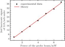
According to Eqs. (7) and (8), a modulation is added to the x-direction coils, whose frequency is 10 Hz and amplitude is 160 pT. The lock-in amplifier is then used to measure the first harmonic, which is proportional to the magnetic field gradient Bg. However, this measurement would introduce a large error, owing to the transmittance of the probe beam being different along the cell, which is caused by the non-uniform thickness of the cell’ s wall and the attachment of the alkali atoms to the cell’ s wall. To demonstrate this clearly, we measure the second harmonic signal, which is proportional to the initial intensity I0 according to Eq. (10), the experimental result is shown in Fig. 2.
 | Fig. 2. The second harmonic signal of the lock-in amplifier, which is proportional to the power of the probe beam as predicted by Eq. (10). |
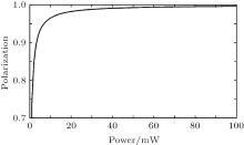
If the alkali atoms are not fully polarized, the electron polarization along the pump beam would be non-uniform. According to Eqs. (2) and (5), we perform a simulation of the electron polarization as a function of pumping laser power, and the result is shown in Fig. 3.
 | Fig. 3. Simulation of the electron polarization as a function of pump laser power, showing that the polarization of the potassium increases with the augmentation of the pump beam power, and the polarization is almost 1, when the pumping laser power is larger than 60 mW. |
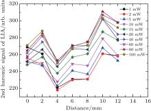
By adjusting the linear translation stage in steps of 2 mm, the probe beam could be launched at different but parallel offset positions along the z direction. The measurement is repeated with varying the power of the pump beam from 1 mW to 100 mW. As shown in Fig. 4, with different powers of pump beam the second harmonic signals are almost parallel to each other, and the different offsets are caused by unequal scale factor of the magnetometer due to the different powers of the pump beam. As the power of the pump beam is increased, the polarization rate of the alkali atoms increases. According to the experimental result, the initial intensity I0 is not a constant at the different points of the cell. For an ideal cell, whose transmissivity to the probe beam is constant, the experimental curves should be constant with different distances. However, as shown in Fig. 4, the curves decay in the middle and at two ends. The decays at two ends are due to partial blocking of the probe beam by the magnetic shield. The signal fluctuation at the location of 4 mm– 8 mm is caused by the attachment of the alkali atoms in the middle of the cell, the cell used in this experiment is shown in Fig. 5.
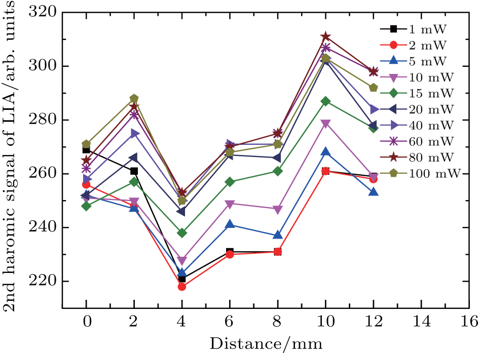 | Fig. 4. The second harmonic signal of the lock-in amplifier with different locations of the probe beam along the z direction. The different offsets of the curves are due to the unequal scale factor caused by different polarization rates. Moreover, when the pump beam’ s power is larger than 60 mW, the alkali atoms are almost fully polarized, and the curves almost overlap. |
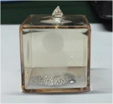
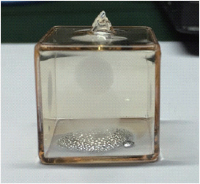 | Fig. 5. Fluctuation in Fig. 4, which is caused mainly by the attachment of the alkali atoms to the cell’ s wall, as shown in this figure, more alkali atoms are attached to the center of the cell’ s wall, which can reduce the power of the probe beam considerably after passing through the center of cell. |
Directly demodulating the first harmonic signal to measure the magnetic field is frequently used. However, the inhomogeneity in the transmissivity of the cell to the probe beam makes this method unable to measure the magnetic field gradient precisely. To solve the problem, the measurement method needs to be modified. According to Eq. (8), when a calibrating magnetic field Bc is applied in the z direction, we find

When the calibration magnetic field is applied to the positive direction of the z axis, an output signal can be acquired, and then we change the sign of the calibration magnetic field, which means that along the negative direction of the z axis, an additional output signal can be acquired. The former output is subtracted from the latter one, resulting in the elimination of the magnetic field gradient and the light shift, the remainder is proportional to 2Bc. Using this method, the scale factor between the output signal and the value of the magnetic field along the z direction can be determined.
The light shift can be treated as fictitious magnetic field, which has considerable effects on magnetic field gradient measurement. Whereas, according to Eq. (6), the frequency of the pump beam is locked to the resonance of the potassium’ s D1 line to suppress the light shift. However, the light shift cannot be ideally attenuated to zero. Furthermore, when the pump beam with low intensity propagates through the cell, the intensity of the pump beam is non-uniform along the z direction, which causes the light shift gradient. The light shift gradient will affect the measurement of the residual magnetic field in the magnetic shield. According to Eq. (6), the direction of the light shift is determined by the photon spin vector of the pump beam. For a σ + -polarized pump beam (s = + 1), the light shift is along the negative direction of the z axis. For a σ − -polarized pump beam (s = − 1), the light shift is along the positive direction of the z axis. After each measurement in which the probe beam propagates from one side of the cell to another side, the σ + -polarized pump beam is changed into σ − , and the measurement is repeated. The magnetic field measured with σ + -polarized pump beam is Bg(z) − BLS(z), and for σ − -polarized pump beam is Bg(z) + BLS(z). Therefore, the magnetic field caused by the residual magnetic field and the light shift can be measured independently.
The calibrating magnetic field along the z direction used in the experiment is set to be approximately 1.6 nT, i.e., Bc ≈ 1.6 nT. The residual magnetic field is then measured by varying the pump beam power from 1 mW to 100 mW. As shown in Fig. 6, when the pump beam power is below 60 mW, the alkali atoms are not fully polarized, which causes inhomogeneous absorption rate of the pump beam as the pump beam propagates through the cell. The non-uniform power of the pump beam results in the light shift gradient. The experimental results of the magnetic field gradient are not accurate with using a low pump beam power. As the power of the pump beam increases, it becomes evident that when the power of the beam is larger than 60 mW, the alkali atoms are fully polarized by the pump beam. When the pump beam power is larger than 60 mW, the measurement results of the magnetic field gradient are almost similar to each other and the differences between them are within 0.25 nT. With a high pump beam power, the light shift should be constant through the cell. However, there is a small offset between the experimental data with pump beam powers of 60 mW, 80 mW, and 100 mW, which may be due to the small deviation of the scale factor calibration with a high pump power. However, the offset does not affect the measurement of the residual magnetic field gradient.
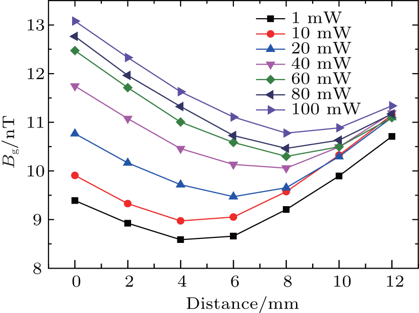 | Fig. 6. Experimental result of the residual magnetic field along the z direction. The measurement of the magnetic field with low pumping power is inaccurate due to the light shift gradient and inhomogeneous polarization rate through the cell. |
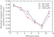
In such a case, the light shift gradient can be suppressed with a high pump beam power. The residual magnetic field gradient is measured when the power of the pump beam is larger than 60 mW, which should ensure that the alkali atoms are fully polarized. As shown in Fig. 7, the magnetic field gradient in the magnetic shield is less than 0.4 nT/mm, and there is a minimum magnetic field gradient between 8 mm and 10 mm, and the minimum gradient is approximately 0.075 nT/mm. The precision of the magnetic field gradient measurement is better than 0.03 nT/mm, and the spatial resolution of the magnetic field gradient measurement inside the magnetometer cell is approximately 2 mm.
 | Fig. 7. Magnetic field gradients along the z direction, measured with pump beam’ s power of 60 mW (solid circle), 80 mW (solid triangle), and 100 mW (solid square). |
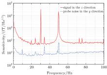
The SERF magnetometer is the most sensitive to the magnetic field in the y direction, and is insensitive to the magnetic field in the z direction, with all residual magnetic fields well compensated. However according to Eq. (3) we can apply a bias or modulation magnetic field to the x direction to make the SERF magnetometer sensitive to the magnetic field in the z direction. We set the pump laser power to be 20 mW and probe laser power to be 1 mW, a 3.2-nT bias magnetic field is applied to the x direction to make the SERF magnetometer sensitive to the magnetic field in the z direction. Then a 22-pT calibration magnetic field is applied to the z direction. As shown in Fig. 8, a sensitivity of 40 fT/Hz1/2 is achieved in the z direction, in contrast the probe noise in the y direction is 5 fT/Hz1/2. The sensitivity of the SERF magnetometer in the z direction is worse than the sensitivity we have achieved in the y direction with optimizations before in Ref. [20]. Nonetheless, the advantage of the SERF magnetometer which is sensitive to the magnetic field in the z direction is that it can be used in magnetic field gradient measurement in the z direction and light shift measurement along the pump beam.
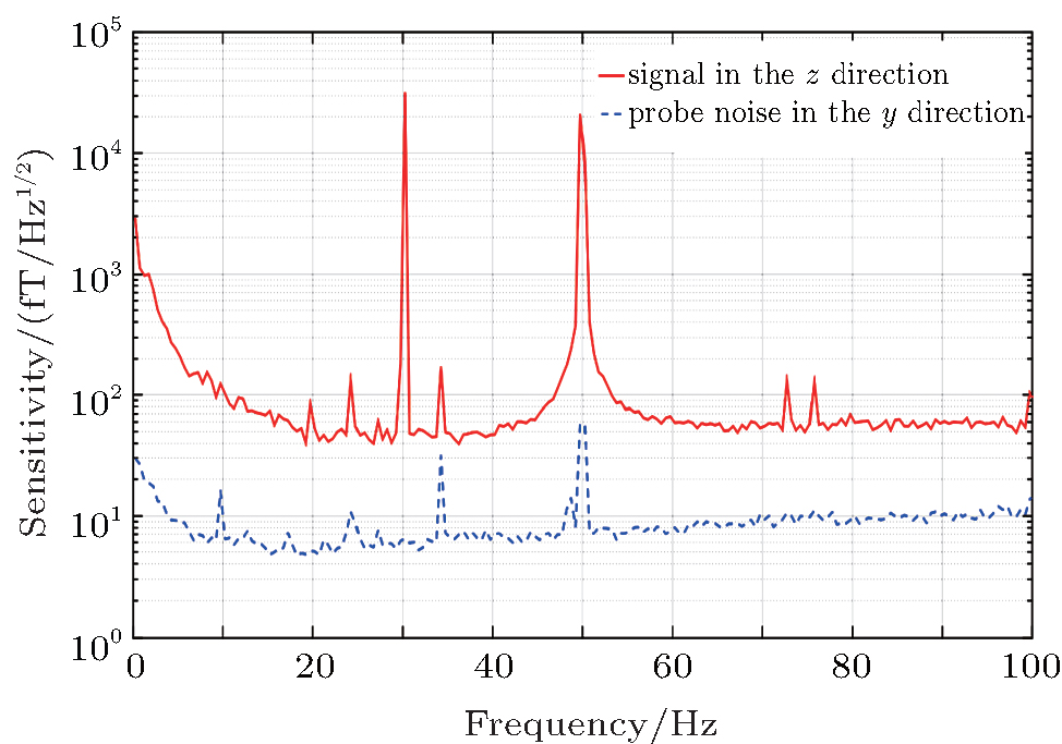 | Fig. 8. Spectra of SERF magnetometer with 30-Hz calibration magnetic field in the z direction, the sensitivity in the z direction is 40 fT/Hz1/2, and the probe noise in the most sensitive axis is 5 fT/Hz1/2. |
We demonstrate a method of measuring an in-situ magnetic field gradient along the pump beam in the magnetic shield. Demodulating the first harmonic signal by lock-in amplifier is a frequently used method to determine the magnetic field. The first harmonic signal is proportional to the intensity of the probe beam. However, due to the inhomogeneous thickness of the cell’ s wall and the attachments of the alkali atoms to the cell’ s wall, the transmissivity of the cell to the probe beam along the pump beam is always inhomogeneous. To solve this problem, we use a calibrating signal to calibrate the magnetometer’ s sensitivity in each moving step. Furthermore, we demonstrate that the light shift and its gradient will reduce the accuracy of the magnetic field gradient measurement. As proposed in this paper, the light shift can be reduced by locking the pump beam to the resonance frequency and measuring the residual magnetic fields with σ + - and σ − -polarized pump beams. The light shift gradient can be suppressed by a relatively high power pump beam, which makes the alkali atoms fully polarized. Finally, we demonstrate the measuring of the magnetic field gradient by using SERF magnetometer, and the precision is better than 30 pT/mm. The sensitivity of the SERF magnetometer is optimized when the polarization equals 1/2.[7] The light shift can be reduced by operating the pump beam in resonance. However, the polarization of the alkali atoms cannot be kept to be 1/2 through the cell as the partially-polarized atoms absorb the pump beam in resonance dramatically.[23] The light shift gradient and polarization gradient measurement will be meaningful to the optimization of the SERF magnetometer. The future work will examine the measuring of the light shift gradient and the polarization gradient along the pump beam.
| 1 |
|
| 2 |
|
| 3 |
|
| 4 |
|
| 5 |
|
| 6 |
|
| 7 |
|
| 8 |
|
| 9 |
|
| 10 |
|
| 11 |
|
| 12 |
|
| 13 |
|
| 14 |
|
| 15 |
|
| 16 |
|
| 17 |
|
| 18 |
|
| 19 |
|
| 20 |
|
| 21 |
|
| 22 |
|
| 23 |
|