The mechanical property of semiflexible biopolymers plays crucial roles in the structure and function of biological materials. For instance, it affects how a double-stranded DNA (dsDNA) wraps around histones. To have a complete understanding of the properties of biopolymers, in general it requires a comparison between experimental observations and theoretical predictions, and recent progresses in experimental techniques have provided powerful tools to manipulate a single biomolecule, which make it possible to do a direct comparison between experiment and theory for a single biopolymer. In theoretical studies, a semiflexible biopolymer is often modeled as an elastic filament. The simplest model for a semiflexible biopolymer is the wormlike chain (WLC) model, which views a biopolymer as an inextensible chain with a uniform bending rigidity but a negligible cross section. It has been reported that the WLC model describes well the entropic elasticity of an intrinsically straight dsDNA.^{[1– 3]} The term “ intrinsically straight" means that the ground state configuration (GSC) of the filament is a straight line or the intrinsic curvature of the filament is zero. As a consequence, in the WLC model the extension of a chain is always a smooth function of applied force, regardless of temperature. However, semiflexible biopolymers are not always intrinsically straight, and there are many intrinsically curved biopolymers owing to the heterogeneous sequence.^{[4– 8]} An example is that the special sequence orders favor a finite intrinsic curvature for dsDNA, such as that the tandem sequence repeats of adenine tracts (A-tracts) can yield a constant intrinsic curvature in dsDNA.^{[6, 7]} It was reported that the WLC model fails to account for the property of intrinsically curved biopolymers even when there is no external force.^{[4– 8]} Moreover, it has been shown that under external force and torque, an intrinsically curved and twisted biopolymer can form a stable helix and the extension of the helix can undergo a discontinuous transition with varying force.^{[9– 11]} It is also clear that adding a nonvanishing intrinsic torsion alone to the WLC model cannot change the smooth variation in extension if we do not fix the initial tilting angle and cross section of the chain, or if the polymer is rather long so that the effect of the boundary condition (BC) becomes negligible. A question is then interesting, i.e., whether a nonvanishing intrinsic curvature alone is enough to induce a discontinuous transition in extension. In this work we perform Monte Carlo (MC) simulation in lattice systems to help to clarify this question. On the other hand, many experiments for semiflexible biopolymer are performed in a two-dimensional (2D) environment so that the property of biopolymers in 2D has attracted growing interest.^{[8, 12– 18]} Therefore, for simplicity we focus on the 2D lattice systems in this work.

A semiflexible biopolymer is often modeled as a filament. In the 2D case, the configuration of a filament is determined by its tangent vector, t ≡ dr/ds = {cosϕ , sinϕ }, to its contour line, where r = (x, y) is the locus of the filament, s is the arclength and ϕ (s) is the angle between the x axis and t. Applying a uniaxial force (along the x axis) F at s = L, we can write the elastic energy of an intrinsically curved filament as^{[8, 12, 13]}

where k is the bending rigidity, L is the contour length and a constant so that the filament is inextensible, is the signed curvature and c̃ is the intrinsic one. c̃ ≠ 0 means that when F = 0, the GSC (or the spontaneous configuration, i.e., the configuration with the lowest energy) of the filament is a curve of curvature c̃ . c̃ can be s-dependent, but for simplicity in this work we consider only constant c̃ . Without loss of generality, we also assume c̃ > 0 and F > 0.

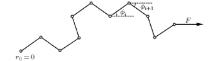
The closed form relation of extension and force for the continuous model under a low or strong F has been found using a series expansion method.^[13] However, to find a closed form solution for the mechanical property of the system under a moderate F and at T > 0 does not seem to be possible. Therefore, to explore this problem, we discretize the model and perform MC simulation method with the Metropolis algorithm in triangle and square lattice systems. In the discrete model, a filament consists of N straight segments of length l₀ joined end by end, as sketched in Fig.  1. Replacing ϕ by (ϕ _{i+ 1}− ϕ _i)/l₀ in Eq.  (1), the reduced energy, ℰ _N, can be written

where k_B is the Boltzmann constant, c ≡ c̃ l₀, κ ≡ k/l₀k_BT, and f ≡ Fl₀/k_BT. We also scale length by l₀ so and the relative extension is defined as z_N = 〈 x_N〉 /N, where 〈 · · · 〉 denotes the thermal average or the configurational average. When c = 0, it is reduced into the WLC model. A straight line in the model is given by Δ ϕ _i = 0 for i = 1, … , N − 1.

Fig.  1.

	Figure Option ViewDownloadNew Window
	Fig.  1. Schematic diagram of the discrete model.

In the present work we study both triangle and square lattices. In a real system, Δ ϕ _i ≡ ϕ _{i+ 1}− ϕ _i = Φ and Δ ϕ _i = 2π + Φ are indistinguishable, but − Δ ϕ _i and Δ ϕ _i are different when c ≠ 0, so we limit π ≥ Δ ϕ _i > − π . Consequently, there are six possible values of Δ ϕ _i in a triangle lattice system (TLS), i.e., Δ ϕ _i = − 2π /3, − π /3, 0, π /3, 2π /3, and π . Similarly, there are four possible values of Δ ϕ _i in a square lattice system (SLS), i.e., Δ ϕ _i = − π /2, 0, π /2, and π . Note that the value of ϕ _i is still unlimited in simulation.

In MC simulation, the initial configurations are set randomly. We equilibrate every sample from 2 × 10⁶ to 5 × 10⁶ Monte Carlo steps (MCS) before performing the averaging. The thermal average for a sample is taken from 1 × 10⁷  MCS to 5 × 10⁷  MCS, and the larger the N or κ or c, the more the MCS. This is because the thermal fluctuation becomes larger with increasing N or κ or c. Moreover, we take N = 20, 50, 100, 150, 200, 250, 300 to examine the finite size effect. c = 0.1, 0.2, 0.3, 0.4, 0.5, 0.7, 0.9 and κ = 1, 2, 4, 6, 8 in MC simulation. We do not consider a larger c because it is impractical. We also do not consider a larger κ because it results in a very large fluctuation. The large fluctuation should result from the existence of metastable states (i.e., the states with a local minimum energy), since a larger bending rigidity can result in a higher energy barrier between different states and it follows that the system may be trapped longer in a metastable state. The thermodynamical limit in this work means that we keep both l₀ and c as constants but let N → ∞ so that the total length L = Nl₀ → ∞ .

We also perform the exact enumeration to study the lattice systems. In exact enumeration, the length of the chain is taken up to N = 12 in both systems. We do not report the results obtained from the exact enumeration method separately in this work because the lengths used in the exact enumeration are still too short to make any reliable conclusion and these results are in fact indistinguishable from that obtained from MC simulation, but at least the agreement between the two methods provides a robust evidence on the reliability of the MC simulation.

At a finite temperature, the fluctuation suppresses sharp transition for a finite-size system. Therefore, to examine the occurrence of phase transition and to identify the nature of transition, one often has to evaluate the finite-size effects. For this purpose, we study the specific heat 𝓒 _N, the stretching modulus μ _N, and the fourth-order cumulants of the order parameter (U_N) and energy (V_N).^[19] They are expressed as

It has been reported that, for the first-order transition, V_N has a minimum at the effective transition point and V_N ≠ 2/3 at the transition point f = f^* as N → ∞ .^[19] In contrast, by scaling analysis, it is found that, for higher-order transitions, V_N → 2/3 as N → ∞ even at f^*.^[19] Meanwhile, for sufficiently large N, curves for U_N cross as a function of f at the ‘ fixed point’ value U^* and the location of the crossing ‘ fixed point’ gives a critical point. Moreover, by scaling analysis, when N → ∞ , U_N → 2/3 if f > f^*, and U_N → 0 if f < f^*; at f^*, U_N tends towards a universal value.

We should point out that at f = 0, from Eq.  (2), for the TLS with c ≥ c^* = π /6, the GSC of the filament is a curve with the smallest (Δ ϕ _i − c)² and so does for small f owing to c² ≥ (π /3− c)² in this case. We can see this point more clearly by examining the simplest case with N = 2 so ℰ = κ /2(Δ ϕ ₁ − c)² − f(cosϕ ₁+ cosϕ ₂). In this case, clearly the bending term dominates the energy when f is small. Therefore, taking a small f and c > c^*, such as c = π /3, we find that in the GSC ϕ ₁ = 0, Δ ϕ ₁ = ϕ ₂ = π /3, and ℰ = − 1.5 f. The first excited state is given by ϕ ₁ = ϕ ₂ = 0 = Δ ϕ ₁ which represents a straight line and ℰ = π ²κ /18 − 2 f. On the other hand, under very large f, clearly the GSC of the filament is a straight line. Owing to the discrete model in ϕ _i and Δ ϕ , there is an energy gap between two GSCs (for small and large f, respectively) in the lattice system and such a gap should favor a sharp transition in z_N when we increase f. In contrast, when c < c^*, at any f the GSC of the filament is a straight line and there are also energy gaps between the GSC and the excited states. For instance, when N = 2, if c = π /9 < c^*, the GSC requires ϕ ₁ = ϕ ₂ = 0 = Δ ϕ ₁ and ℰ = π ²κ /162 − 2 f, and the first excited state is given by ϕ ₁ = 0, Δ ϕ ₁ = ϕ ₂ = π /3, and ℰ = 2π ²κ /81 − 1.5 f. Intuitively, these energy gaps would disfavor a sharp transition. The same arguments can be applied to the SLS but the critical curvature becomes c^* = π /4. Consequently, if there were no phase transition in the lattice system when c > c^*, we could safely conclude that there was neither in the off-lattice system. Meanwhile, since when c < c^* the GSC in the lattice systems is always a straight line, intuitively the behavior of the filament would be similar to that of the case with c = 0. Therefore, if there is still a phase transition when c < c^*, we expect that the same phenomenon occurs in the off-lattice system. These are also the important reasons why we study lattice systems first, besides it is easier to perform the simulation.

We have already presented an informal and incomplete brief report for the results in the lattice systems.^[20] In this paper we present the detailed results.

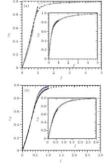
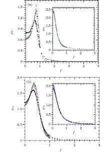
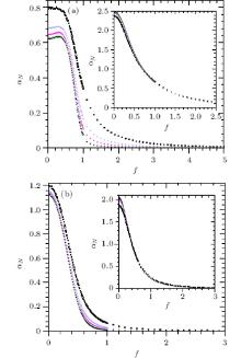
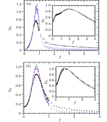
Firstly, when either κ or c is small, we find that z_N is a simple smooth concave function of f, or the larger the f, the slower the increment rate in z_re at any f. This is a natural result since a small c means that the model is close to the WLC model so that the results should also be similar. Meanwhile, a small κ means that the filament is rather flexible so that the bending energy or curvature is less important at finite T. We should note that when κ = 0 the model is reduced into the freely jointed chain model, and it is well known that the extension of the freely jointed chain model is a smooth concave function of force. The insets in Fig.  2show two typical results with κ = 2, c = 0.2 for TLS and κ = 1, c = 0.1 for SLS. Correspondingly, μ _N decreases monotonically with increasing f, as shown in the insets of Fig.  3. In these cases, the finite size effect is also rather weak so that the results with N = 100 and N = 300 are almost indistinguishable. Therefore, there is no phase transition in z_N in these cases.

Fig.  2.

Figure Option ViewDownloadNew Window

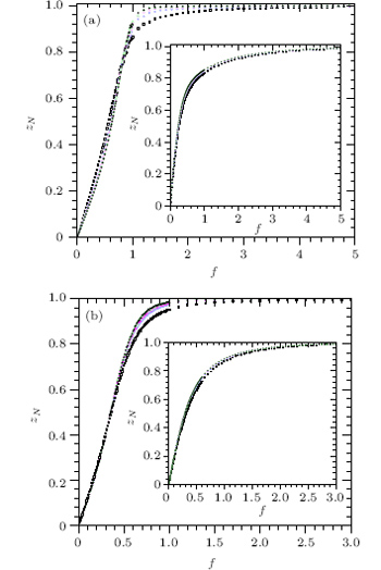Fig.  2. (a) zN versus f for a triangle lattice when κ = 8, c = 0.5 and κ = 2, c = 0.2 (inset). The lengths of the filaments are N = 20 (black empty-square), 50 (blue empty-circle), 100 (magenta filled-triangle), 200 (green empty-triangle), 300 (black filled-circle). (b) zN versus f for a square lattice when κ = 6, c = 0.7 and κ = 1, c = 0.1 (inset). The symbols are the same as those in panel  (a). Reduced units are used.

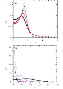
However, large κ or c results in completely different results. When κ > 4 and c > 0.2, we find that the curve of z_re versus f is no longer a simple concave function. More exactly, at low f it is a convex function but at large f it is a concave function. Though z_N still increases monotonically with increasing f, there exists an inflection point, denoted by f = f_i, in which the curve of z_re versus f changes from being convex to concave. When f < f_i, the larger the f, the larger the increment rate in z_re, as shown in Fig.  2 for both the lattice systems. But when f > f_i, the larger the f, the smaller the increment rate in z_re. Consequently, μ _N has a sharp peak at f = f_i and the height of the peak increases clearly with increasing N, as shown in Fig.  3. We also find the same behavior for 𝓒 _N, as shown in Fig.  4. The growing sharp peaks in μ _N and 𝓒 _N clearly indicate the existence of a phase transition in the thermodynamical limit, i.e., the peak values of μ _N and 𝓒 _N should approach infinity when N → ∞ , and the critical force f^* = lim_{N → ∞} f_i. Moreover, the unique peak at a large N in μ _N and 𝓒 _N also suggests that the transition is a single step. We should also note that even with small κ and c, we still observe some broad peaks in 𝓒 _N, but the heights of these peaks grow very slowly with N and there is no corresponding peak in μ _N, as shown in the insets of Figs.  3 and 4. Therefore, these broad peaks of 𝓒 _N correspond to the change in modes, such as from linear to nonlinear relations in z_N(f), instead of a phase transition in z_N(f).

Fig.  3.

	Figure Option ViewDownloadNew Window
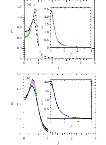	Fig.  3. (a) μ N versus f for a triangle lattice when κ = 8, c = 0.5 and κ = 2, c = 0.2 (inset). (b) μ N versus f for a square lattice when κ = 6, c = 0.7 and κ = 1, c = 0.1 (inset). The symbols are the same as those in Fig.  2. Reduced units are used.

Furthermore, our results show that at the same κ and N, the larger the c, the larger the f^*, as shown in Fig.  5. This should be a natural result since after transition, the filament always becomes nearly straight, but larger c means that the filament is more likely to be in a curved state, so to straighten out it requires a larger force. This result is also the same as that observed in the off-lattice system.^{[20, 21]}

Fig.  4.

	Figure Option ViewDownloadNew Window
	Fig.  4. (a) 𝓒 N versus f for a triangle lattice when κ = 8, c = 0.5 and κ = 2, c = 0.2 (inset). (b) 𝓒 N versus f for a square lattice when κ = 6, c = 0.7 and κ = 1, c = 0.1 (inset). The symbols are the same as those in Fig.  2. Reduced units are used.

Fig.  5.

	Figure Option ViewDownloadNew Window
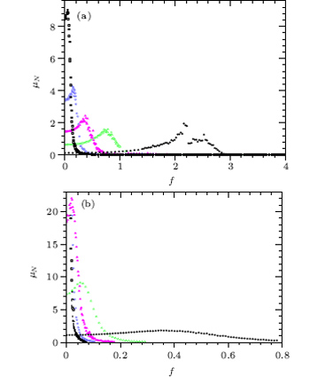	Fig.  5. (a) μ N versus f for a triangle lattice when κ = 8 and c = 0.2 (black empty-square), 0.3 (blue empty-circle), 0.4 (magenta filled-triangle), 0.5 (green empty-triangle), 0.7 (black filled-circle). N = 300 in all the cases. (b) μ N versus f for a square lattice when κ = 6 and c = 0.2, 0.3, 0.4, 0.5, 0.7. The symbols are the same as those in panel  (a). Reduced units are used.

On the other hand, at the same c and N, the relationship between f^* and κ is dependent on the lattice structure. In TLS, we find that when c < c^*, f^* is not a monotonic function of κ . More exactly, f^* increases with increasing κ first, and then decreases with increasing κ , as shown in Fig.  6(a). In contrast, when c > c^*, a larger κ always results in a larger f^*. In SLS, we find that when c < c^*, f^* always decreases with increasing κ , as shown in Fig.  6(b). But when c > c^*, a larger κ also results in a larger f^*. The structure-dependent behavior is quite different from that observed in the off-lattice system, ^{[20, 21]} and indicates that the existence of energy gaps can accelerate the transition. This should be due to the fact that when c < c^* and κ are large, the energy gap between GSC and the excited state also becomes large so that the system is easier to collapse to the GSC.

Fig.  6.

	Figure Option ViewDownloadNew Window
	Fig.  6. (a) μ N versus f for a triangle lattice when c = 0.5, and κ = 2 (black empty-square), 3 (red diamond), 4 (blue empty-circle), 6 (magenta filled-triangle), 8 (black filled-circle). N = 300 in all the cases. (b) μ N versus f for a square lattice when c = 0.5, and κ = 2, 4, 6, 8. The symbols are the same as those in panel  (a). Reduced units are used.

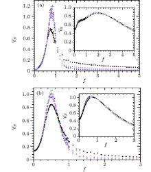
To have a complete picture, we also evaluate and e_N ≡ 〈 ℰ _N〉 /N. We find that α _N has rather different behavior between TLS and SLS, as shown in Fig.  7. In TLS, when κ or c is small so that no transition occurs, α _N decreases monotonically with increasing f, as shown in the inset of Fig.  7(a). However, when κ or c is large, we find that there is a platform in z_N when even when N is small, and it follows a rapid drop in z_N near to , as shown in Fig.  7(a). The finite size effect is also very clear in this case so it offers another evidence for a sharp transition. In contrast, in SLS, we do not find the platform even up to κ = 8, c = 0.9, and N = 300. In SLS, α _N exhibits only a strong finite size effect when κ or c is large, as shown in Fig.  7(b). The different behaviors of α _N between the two systems should be resulted from the difference in the energy gaps between the ground state and the excited states. The energy gap in the SLS is larger than that in the TLS, thus at finite T it leads to a faster collapse of the excited states into the ground state which is a straight line, and depresses the fluctuation in y_N.

Fig.  7.

	Figure Option ViewDownloadNew Window
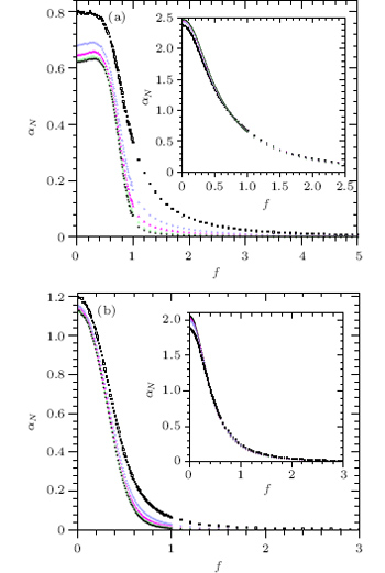	Fig.  7. (a) α N versus f for a triangle lattice when κ = 8, c = 0.5 and κ = 2, c = 0.2 (inset). (b) α N versus f for a square lattice when κ = 6, c = 0.7 and κ = 1, c = 0.1 (inset). The symbols are the same as those in Fig.  2. Reduced units are used.

On the other hand, we do not find any qualitative difference in the mean energy, e_N, between the samples with and without phase transition, as shown in Fig.  8. Especially, near to the critical force we do not observe any sharp change in e_N for the samples having phase transition. Therefore, e_N provides little information for the transition in the present work and it may deserve further exploration. However, we find that at large f, e_N decreases almost linearly with increasing f in all the cases. In this regime, the filament is almost straight, so that the energy dominates the physical property of the system and the entropy plays little role. It follows that z_N varies very slowly with varying force, in agreement with the results shown in Fig.  2.

Fig.  8.

	Figure Option ViewDownloadNew Window
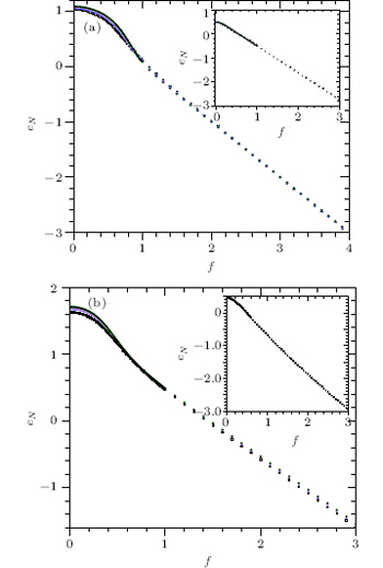	Fig.  8. (a) eN versus f for a triangle lattice when κ = 8, c = 0.5 and κ = 2, c = 0.2 (inset). (b) eN versus f for a square lattice when κ = 6, c = 0.7 and κ = 1, c = 0.1 (inset). The symbols are the same as those in Fig.  2. Reduced units are used.

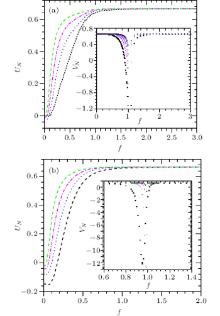
Furthermore, as shown in the inset of Fig.  9, we find that for the samples having a phase transition, V_N ∼ 2/3 at either small f or large f, but V_N has a minimum which is smaller than 2/3 at a moderate f. Meanwhile, in all the cases, when N > 20 we do not find any intersection point in U_N, and U_N → 2/3 only when f is rather large, as shown in Fig.  9. The behaviors of U_N and V_N suggest that the phase transition is of the first-order one.^[19]

Finally, since we observe the discontinuous transition in z_N in both lattice systems even when c < c^*, we can conclude that the transition is dominated by the magnitude of c, instead of the energy gaps in the lattice systems. Consequently, we can also expect that the same phenomenon occurs in the off-lattice system, agreeing with the findings in the off-lattice system.^{[20, 21]} An energy gap is not necessary for the phase transition but it can accelerate the collapse of configurations into the GSC and make the transition easier.

Fig.  9.

	Figure Option ViewDownloadNew Window
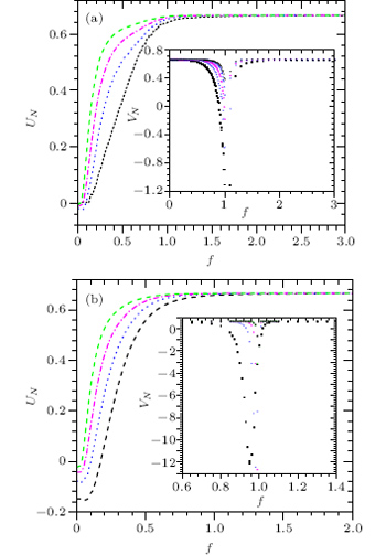	Fig.  9. (a) UN and VN (inset) versus f for a triangle lattice when κ = 8 and c = 0.5. (b) UN and VN (inset) versus f for a square lattice when κ = 8 and c = 0.5. For UN, the lengths are N = 20 (black short-dashed), 50 (blue dotted), 100 (magenta dash-dotted), 200 (green dashed), and 300 (black solid). For VN, the symbols are the same as those in Fig.  2. Reduced units are used.

In summary, at finite temperature we find that an intrinsic curvature of sufficient magnitude can induce a discontinuous transition in extension of a semiflexible biopolymer in the thermodynamical limit. This conclusion is valid in both triangle and square lattice systems, and agrees with the findings in the off-lattice system.^{[20, 21]} The critical force increases with the increasing intrinsic curvature. However, the relationship between the critical force and the bending rigidity is dependent on the structure of the lattice. In a triangle lattice system, when the intrinsic curvature is smaller than a critical value, the critical force increases with the increasing bending rigidity first, and then decreases with the increasing bending rigidity. In a square lattice system, however, the critical force always decreases with the increasing bending rigidity. In contrast, when the intrinsic curvature is greater than the critical value, the larger bending rigidity always results in a larger critical force in both lattice systems. Our results also suggest that the intrinsic curvature dominates the transition and the energy gaps in the lattice system only help to accelerate the transition.