Gilbert damping in the layered antiferromagnet CrCl₃

Introduction

Antiferromagnets (AFMs) allow designing high-speed and robust spintronic devices due to the advantages of zero net magnetization and high resonant frequency up to THz.^[1–6] Studies on spin-transfer torque^[7–11] and anisotropic magnetoresistance^[12,13] explored the rich physics and advanced the potential applications by controlling and detecting the magnetic order in antiferromagnets. Further development and applications of devices based on antiferromagnetic materials require a more comprehensive understanding of antiferromagnetic dynamics. But different from ferromagnetic dynamics, there is little known about antiferromagnetic dynamics^[14–16] due to the more complex internal structures and higher resonant frequencies requiring terahertz techniques to detect.^[1,17,18]

To describe the magnetization dynamics of antiferromagnetic systems, a key issue is to find the proper form of damping. Damping represents the dissipation of energy in the magnetic system, which affects the response speed of magnetic devices. It is inextricably linked to many magnetic phenomena such as spin pumping, spin transfer, and domain wall motion,^[19,20] and plays an important role in the study of magnetic dynamics. In ferromagnetic systems, there have been a lot of detailed studies on magnetization dynamics with damping,^[21–29] and a complete theory has been formed to describe the ferromagnetic dynamics.^[22,25] Generally speaking, the magnetization dynamics in a ferromagnetic system is determined by the Landau–Lifshitz–Gilbert (LLG) equation^[22,25]1m˙=γm×Heff−αm×m˙,where H_eff is the effective field including the external field, the exchange field and the anisotropy field. γ is the gyromagnetic ratio. α is the Gilbert damping constant. The first term on the right-hand side of Eq. (1) determines the precessional motion of the magnetic moment in the ferromagnet around the effective field. The second term is the Gilbert damping which makes the direction of the magnetic moment gradually align to the effective field. The linewidth of the ferromagnetic resonance derived from the LLG equation shows a linear relationship with frequency ΔH–ω,^[30] which produces a good agreement with extensive experiments in the ferromagnetic systems.^[30–33] So the magnetic damping in ferromagnets is usually investigated by linewidths due to the linear relationship between ferromagnetic resonance linewidths and damping.^[30–33]

Although there has been a great deal of research in antiferromagnetic dynamics, there is still not a universally accepted dynamic equation until now. In the 1950s, Kittel applied the Landau–Lifshitz equation to the two sublattices of antiferromagnet and calculated the resonance frequencies of AFMs.^[34,35] Following the classical Lagrangian approach that has previously been employed for FMs by Gilbert,^[22] Kamra et al. used Lagrangian equations with Rayleigh dissipation to describe the antiferromagnetic dynamics in 2019,^[36] and successfully predicted the enhancement of the dissipation rate of ferrimagnets at the compensation point, which has a good agreement with recent experiments.^[36,37] The same theory was used by Yuan et al. to find a significant effect of the dissipation moment on the magnon lifetime and domain wall motion.^[38] These studies are all for the case of collinear magnetization with an external magnetic field less than the spin-flop field. In a non-collinear magnetization case, the damping process would be expected to be different because the asymmetry between the sublattices has an impact on dynamical spin exchange interaction during the antiferromagnetic resonance (AFMR). For example, in a layered antiferromagnet CrCl₃, the magnetization from each layer can be easily aligned to a non-collinear case by an external magnetic field due to the relative weak coupling.^[39]

In this work, we studied the damping evolution of both acoustic and optical magnetic resonance modes in CrCl₃, again starting from the Lagrangian equation with Rayleigh dissipation.^[22,36,38] The equations depicting the antiferromagnetic dynamics were established following the method of establishing the LLG equations in ferromagnets using the Lagrangian approach.^[22] We obtained the same antiferromagnetic dynamics equations with Kamra and Yuan’s works.^[36,38] The Gilbert damping parameter was represented by a 2 × 2 matrix containing intralayer as well as interlayer damping terms. Then, we applied this theory to describe the antiferromagnetic resonance in CrCl₃.^[39] The expressions of the linewidths of the optical and acoustic modes were obtained, which predict the linewidth evolution of the optical and acoustic modes with frequency. They both have a non-linear growth but the growth trend of the optical mode is much faster than the acoustic mode. Our experimental data also proved this point. Combining both of our theoretical prediction and experimental observations, we concluded that the nonlinear damping evolution ΔH–ω is a intrinsic nature during the antiferromagnetic resonance and the interlayer Gilbert dissipation plays an important role in the non-linear growth of linewidth because of the asymmetry of the non-collinear magnetization between layers.

The theory of antiferromagnetic dynamics

We consider the simplest antiferromagnet with two sets of sublattices, whose magnetizations are described by M₁ and M₂, respectively. Here we describe this system in the frame of the Lagrangian classical field theory, with introducing the so-called Rayleigh dissipation functional ℛ[M.1,M.2]. Then the Lagrangian equation describing the antiferromagnetic system is given by2ddt∂ℒ∂M.i−∂ℒ∂Mi=−∂ℛ∂M.i,where ℒ=T−U is the Lagrangian, and T and U are the kinetic energy and potential energy of the antiferromagnetic system, respectively. The Rayleigh dissipation function ℛ, which describes the energy dissipation in the magnetization motion, has the following form in the antiferromagnetic system:3ℛ[M.1,M.2]=12∑i,j=1,2ηijM.i⋅M.j.

The parameter matrix η_ij quantities the intralayer and interlayer dissipation rate of each sublattice magnetization motion, and the interlayer dissipation may derive from the spin pumping effect between adjacent layers in AFMs.^[38,40] For the antiferromagnet with two sublattices, the potential energy U=−μ0∑i=12Mi⋅Hi, where Hi is the effective field applied to the i-th sublattice magnetization, and the Lagrange equation can be simplified to4ddt∂T∂M.i−∂T∂Mi=μ0Hi−∑j=1,2ηijM.j.

The kinetic energy of a spin comes from the Berry phase caused by spin motion.^[41] For an antiferromagnet with two sublattices, the kinetic energy can be rewritten as T=−∑i=12AiγMi2∂Mi∂t, where A_i is the magnetic potential corresponding to the i-th sublattice magnetization, which is decided by ∇ × A_i = M_i.^[38] Replacing the kinetic energy term with the above expression in Eq. (4), we can get5M.i=μ0γMi×Hi−γ∑j=1,2ηijMi×M.j.

We find that Eq. (5) has exactly the same form as the LLG equation, with the following transformation:6α=(α11α12α21α22)=γM0(η11η12η21η22),where we have made a simplification |M₁| = |M₂| = M₀, which is very reasonable for antiferromagnets. So far we have obtained the equation describing the antiferromagnetic dynamics, which is equivalent to the theory applied in two-sublattice ferrimagnets at the compensation point in Kamra’s work or Yuan’s theory for AFM system with two sublattices.^[36,38]

But there are still too many parameters in the matrix α. Here we proceed to simplify. Firstly, due to the high symmetry of the two sets of sublattices in the antiferromagnet, this requires that the α matrix is symmetric and the diagonal elements must be equal, namely, α₁₁ = α₂₂, α₁₂ = α₂₁. Secondly, according to the second law of thermodynamics, the entropy of an isolated system does not decrease, so the energy of a system without external energy input does not increase. This implies that the eigenvalues and the elements of the damping matrix α must be non-negative.

When there is only one set of magnetic moments, the term γηijMi×M.j which describes the interaction between the two sets of magnetic moments no longer exists and the equation naturally evolves into the LLG equation in ferromagnet systems.^[22] And if we set η = O, Eq. (5) becomes an equation for an undamped magnetization system, which is equivalent to the Landau–Lifshitz equation in ferromagnets.

Then we apply the theory developed above to describe the antiferromagnetic dynamics in the layered antiferromagnet CrCl₃. In the macro approximation, we assume that the magnetization direction is uniform within each layer in CrCl₃, and use M₁ and M₂ to represent the total magnetic moment of the two different sublattices. As for the selection of the effective field, we use the same form as in the Liu’s paper,^[39] which has been shown to be well suited to describe the antiferromagnetic dynamics in CrCl₃. Thus, the LLG equation in CrCl₃ has the following form:^[34,35,39]7dM1dt=μ0γM1×[H−HEM0M2−(M1⋅z)z]−α0M0M1×dM1dt−α12M0M1×dM2dt,8dM2dt=μ0γM2×[H−HEM0M1−(M2⋅z)z]−α0M0M2×dM2dt−α12M0M2×dM1dt,where H_E is the interlayer exchange field and M₀ is the saturation magnetization, |M₁| = |M₂| = M₀. γ is the gyromagnetic ratio and z is along the crystal c axis perpendicular to sample plane. And α₀ = α₁₁ = α₂₂ is the Gilbert damping parameter in the layer, α₁₂ = α₂₁ is the Gilbert damping parameter between layers, and H = H₀ + h is the external magnetic field, where H₀ is the static magnetic field and h is the rf magnetic field.

The linewidth in the antiferromagnetic resonance

In the work of Kamra and Yuan,^[36,38] they discussed the damping of the right-handed mode and left-handed mode in AFMR when the external magnetic field was applied to the direction of magnetization.^[36,38] Different from the situation they discussed, here we discuss the damping of the optical mode and acoustic mode in CrCl₃. When the magnetic field H₀ is applied in the layer plane and perpendicular to the direction of magnetization, Eqs. (7) and (8) are symmetric around the direction of the external magnetic field. Under a linear approximation, we can solve Eqs. (7) and (8) to obtain two independent modes (optical mode and acoustic mode), which can be excited by the microwave field in certain conditions.^[39] The optical and acoustic modes will form a Lorentzian resonance curve. Their resonant frequencies ω_O and ω_A have the relationship with magnetic field as follows:^[39]9ωO=μ0γ2HEM0cosϕ,10ωA=μ0γ2HE(2HE+M0)sinϕ,where ϕ is the angle of deflection of the magnetization direction under the external magnetic field and has the relationship sinϕ = H/2H_E. This was the work of Liu et al.,^[39] but the effect of damping was neglected in their work and the damping evolution ΔH–ω was not further investigated. We have found the appropriate damping to describe the dissipation of AFM dynamics in CrCl₃, and in this way we obtain the linewidth ΔH as a function of the microwave frequency. Here we do not consider a broaden line width independent of the resonance frequency, which is originated from the multi-domain state as inhomogenous in the real sample.11ΔHO=ω[(α0−α12)M0+2(α0−α12)HEcos2ϕ+2α12M0cos2ϕ]μ0γM01−cos2ϕ,12ΔHA=2HE[(α0−α12)(2HE+M0)+2(α0−α12)HEsin2ϕ+2α12(2HE+M0)sin2ϕ]2HE(2HE+M0).

Equations (11) and (12) constitute the main conclusions of this paper and demonstrate that (i) the variation of linewidth ΔH with frequency in antiferromagnets is not a simple linear relationship, which is very different from the linear relation μ₀ΔH = μ₀ΔH₀ + αω/γ in ferromagnets,^[30] and (ii) the linewidth variation is still different between the optical and acoustic modes, with the linewidth of the optical mode increasing faster than the acoustic mode.

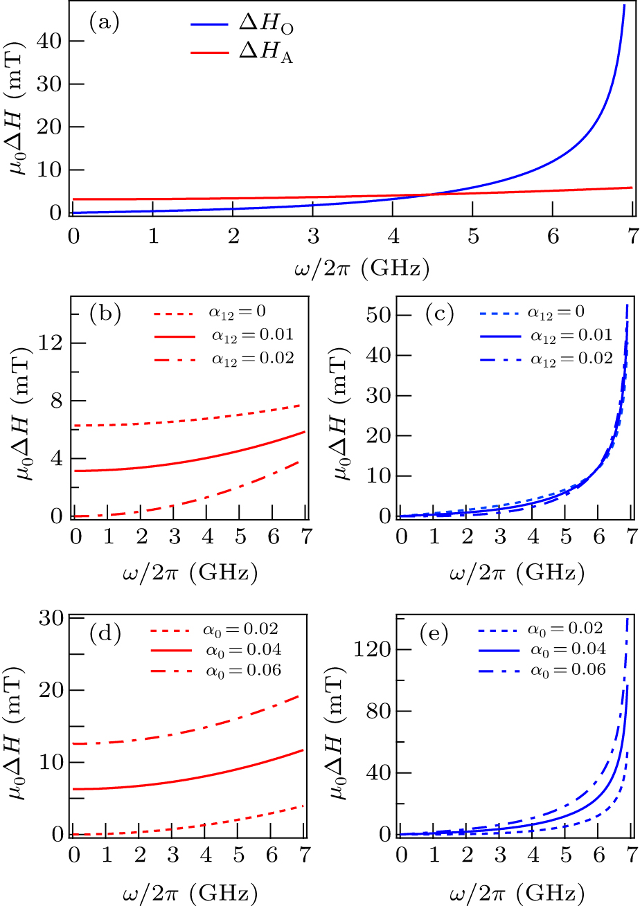
To gain further insight into the results presented in Eqs. (11) and (12), we plot the damping evolution ΔH–ω of the optical and acoustic modes in Fig. 1. The parameters employed in the figure are μ₀H_E = 95 mT, μ₀M₀ = 330 mT and γ = 28/2π GHz/T, which can well reflect the characteristics of antiferromagnets with the weak interlayer coupling, such as CrCl₃. The damping parameter α is around 10⁻² in ferromagnets, such as YIG, and we therefore choose α₀ and α₁₂ to be on the same order of magnitude. And here we do not consider the effect of the non-uniform linewidth. As shown in Fig. 1(a), the linewidths of the optical and acoustic modes both grow nonlinearly with the increase of frequency, but there is a clear difference between them. For the acoustic mode, the linewidth still has a certain value at zero-frequency and grows more slowly, while for the optical mode, the linewidth increases dramatically from zero and surpasses the acoustic mode at around 4.5 GHz. To further investigate the effect of different damping parameters α₀,α₁₂ on the linewidth, we fix α₀ and change α₁₂ in the Figs. 1(b) and 1(c). We do the opposite in Figs. 1(d) and 1(e), and find that in the acoustic mode, the growth rate of linewidth increases with the growth of α₀ or α₁₂, and the linewidth at the zero-frequency increases with the growth of α₀, but reduces with the growth of α₁₂. When α₀ = α₁₂, the linewidth at the zero-frequency will disappear. In the optical mode, the linewidth increases with the growth of α₀ as it does in the acoustic mode. But with the growth of α₁₂, it grows at low frequencies and decreases at high frequencies. Moreover, the linewidth at the zero-frequency is always zero. Then we can get the conclusion that the nonlinear damping evolution ΔH–ω is a consequence of the interlayer interaction during the antiferromagnetic resonance, which is not decided by α₀ or α₁₂ and the interlayer Gilbert dissipation also plays an important role in changing the value of the nonlinear linewidth. We notice that the new damping term α₁₂ will have the effect only when the sublattice is asymmetric, according to the theory of karma.^[36] But in our work, the operation of applying an external magnetic field perpendicular to the direction of magnetization has broken the centrosymmetry, so here the new damping term α₁₂ always exists.

View original graphic| Download| PPT slide

Fig. 1.   The linewidth ΔH as a function of the frequency for the optical mode and acoustic mode. The curves in blue and red depict the optical and acoustic modes, respectively. (a) The curves are calculated according to Eqs. (11) and (12) by setting α₀ = 0.02,α₁₂ = 0.01. For (b) and (c) α₀ = 0.02, α₁₂ = 0, 0.01 and 0.02 correspond to dashed, solid and dash-dotted curves, respectively. α₁₂ = 0.02, α₀ = 0.02, 0.04 and 0.06 correspond to dashed, solid and dash-dotted curves for (d) and (e), respectively.

Experimental results

Based on the above theoretical model, we conducted experiments to investigate the resonance frequency and the damping evolution ΔH–ω of the optical and acoustic modes in antiferromagnet CrCl₃. To measure the AFMR signal of the antiferromagnet CrCl₃, an external magnetic field H = H₀ + h was applied to the CrCl₃/Pt bilayer to drive the antiferromagnetic resonance. The microwave field component h in the y–z plane was applied by placing a coplanar waveguide along the x-axis. The static magnetic field H₀ was applied along the y-axis. The microwave power was 100 mW and the modulation frequency used for lock-in measurement was 8.33 kHz. Thus, the optical mode and the acoustic mode were driven by h_y and h_z, respectively.^[39] In our experiments, the CrCl₃/Pt strip was placed along the x- and y-axis. The microwave transmission intensity was simultaneously measured as a DC voltage through a diode. To perform measurements at low temperatures, the device was placed in a cryogenic chamber.

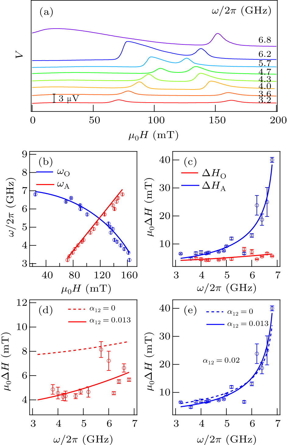
The evolution of AFMR in CrCl₃ is measured in DC voltage by sweeping magnetic field at fixed frequency ω as shown in Fig. 2(a).

View original graphic| Download| PPT slide

Fig. 2.   (a) Evolution of the AFMR in CrCl₃ measured by DC voltage through a diode. The dispersion (b) and the damping evolutions (c) of the optical and acoustic modes in CrCl₃. The damping evolutions with different α₁₂ of the optical (d) and acoustic modes (e) in CrCl₃. The blue curve and the red curve in (b) are plotted according to Eqs. (9) and (10), respectively. The blue and the red curves in (c)–(e) are plotted according to Eqs. (11) and (12), respectively. And the dashed curves different from solid curves are the parameter α₁₂ = 0.

Figure 2(b) shows the results in which the resonant frequencies of the optical and acoustic modes are as a function of the magnetic field H. We use Eqs. (9) and (10) to fit the resonance frequencies.^[39] These fits are shown by the red and blue lines in Fig. 2(b), which represent the optical and acoustic modes, respectively, with fit parameters of μ₀H_E = 95 mT, μ₀M₀ = 330 mT and γ/2π = 28 GHz/T. As shown in Fig. 2(b), with the choice of the above parameters, the fitted curves agree well with our experimental data, both for the optical and acoustic modes. And this result has been confirmed by the work of Liu et al.^[39] But the damping is neglected in their work which is very important to the antiferromagnetic dynamic.

Here we further study the damping evolution ΔH–ω of the optical and acoustic modes, which are shown in Figs. 2(c)–2(e). Then we use Eqs. (11) and (12) with different non-uniform linewidth terms ΔH_O0 and ΔH_A0 to fit the linewidth of the optical and acoustic modes. The parameters H_E and M₀ are fixed, which have been obtained from fitting the resonant frequency above.^[39] These fits are shown by the red and blue solid lines in Figs. 2(c)–2(d), which represent the optical and acoustic modes, respectively. The fit parameters employed are α₀ = 0.02, α₁₂ = 0.013, ΔH_O0 = 3.18 mT and ΔH_A0 = 1.30 mT. As shown in Figs. 2(c)–2(e), in the range of 3 GHz to 7 GHz, our theory agrees very well with the experimental data for the optical, and for acoustic modes, there is a small deviation between the experimental data and the theoretical prediction which may originate from our experiment with large error bar, but the trend of variation between the theoretical and experimental data is the same. The optical and acoustic modes both show a non-linear increase in linewidth with increasing frequency. Moreover, our theory and experiments also show that the optical mode will have a dramatic increase in linewidth with increasing frequency. But for acoustic mode, the increasing trend is more gentle than optical mode as shown in Fig. 2(c). So at high frequencies, the linewidth of optical mode will be much larger than acoustic mode. To further study the role of α₁₂ in damping, we set α₁₂ = 0 in the red and blue dash lines as a contrast in Figs. 2(d) and 2(e), and other parameters are the same as the solid lines. But there is no very huge difference between the dashed lines and solid lines in Figs. 2(d) and 2(e). Although our theory predicts that α₁₂ has a significant effect on linewidth, further experiments are needed to verify that.

Summary

In this work, we have theoretically and experimentally investigated the Gilbert damping evolution ΔH–ω of optical and acoustic mode with frequency in the layered antiferromagnet flake CrCl₃. We discovered that the linewidths of both optical and acoustic modes have a nonlinear positive correlation with frequency in AFMs, which is different from the linear relationship in ferromagnets. We developed suitable damping from the Lagrange equation with the Rayleigh dissipation functional to account for the linewidth of the optical and acoustic modes and predicted nonlinear ΔH–ω relationship for both optical and acoustic modes, which is in agreement with our experimental observations. Combining both our theoretical prediction and experimental observations, we concluded that the nonlinear damping evolution ΔH–ω is a intrinsic nature, which is derived from the interlayer interaction during the antiferromagnetic resonance. Our work provides a method for extracting damping parameters from antiferromagnetic linewidths, allowing a quantitative measure of the magnitude of dissipation in antiferromagnetic resonances.

Acknowledgements

Project supported by the National Natural Science Foundation of China (Grant No. 11774200), the Shandong Provincial Natural Science Foundation, China (Grant No. ZR2019JQ02), and the Youth Interdisciplinary Science and Innovative Research Groups of Shandong University.

Reference

View Option

• By original order
• By published year
• By cited within times
• By Impact factor