Realization of adiabatic and diabatic CZ gates in superconducting qubits coupled with a tunable coupler**

Project supported by the National Natural Science Foundation of China (Grant Nos. 11890704, 12004042, and 11674376), the Natural Science Foundation of Beijing, China (Grant No. Z190012), the National Key Research and Development Program of China (Grant No. 2016YFA0301800), and the Key-Area Research and Development Program of Guang-Dong Province, China (Grant No. 2018B030326001).

Introduction

A programmable superconducting information processor which consists of a two-dimensional array of 53 transmon qubits has been demonstrated to achieve the supremacy for a specific computational task.^[1] A fast, high-fidelity gate scheme is the key to reaching this milestone. For superconducting transmon/Xmon qubits,^[2,3] there are a variety of proposals to realize two-qubit gates which can be divided into three main classes. The first class is implemented with frequency-tunable qubits with the static couplings. Interactions between qubits can be turned on and off by tuning the frequency of qubits. In particular, by tuning the qubits to make the |11〉 state in resonance with |02〉 state, the controlled-Z (CZ) gates can be realized.^[4–8] Furthermore, parametrically modulated qubits make particular states in resonance to realize the iSWAP gate and the CZ gate.^[9] In such schemes, each qubit needs an additional magnetic flux bias line, which makes the circuit complicated when scaling up qubit numbers. The second class is implemented with frequency-fixed qubits and the static coupling strengths.^[10–12] The qubits gates are realized with all microwave driver methods, such as the cross-resonance (CR) gate.^[13–19] This scheme is facing frequency crowding problems, thus limiting the circuit integration. The last class is implemented with frequency-fixed or frequency-tunable qubits coupled with an additional tunable coupler. The general scheme is that two frequency-fixed qubits have a large frequency detuning to eliminate the ZZ interaction which can induce the single qubit gate errors, then parametrically modulated coupler method is used to realize the iSWAP and CZ gates.^[20] A more advantage scheme is to treat the tunable coupler as a switch which can quickly turn on/off the interactions between adjacent qubits.^[21–29] The coupler will turn off the interaction between adjacent qubits when the single qubit gate is implemented. In contrast, two-qubit gates are activated when the coupler turns on the interactions. Another advantage is that qubits do not need large frequency detuning and the frequency crowding problem can also be alleviated.^[1]

By now, the CZ gate fidelity is as high as 99.7%.^[30] Fast gate and low operation errors are two keys to improve the two-qubit gates fidelity. In general, long gate time means more incoherence errors. However, shorter gate time will cause more operation errors. To solve this conflict problem, a fast adiabatic protocol is proposed^[8,31,32] and the gate time is about 30–40 ns. Then, the nonadiabatic gates^[33–35] are found to have fast gate time, which can eliminate the incoherent errors.

Experiments

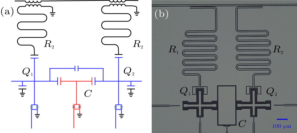
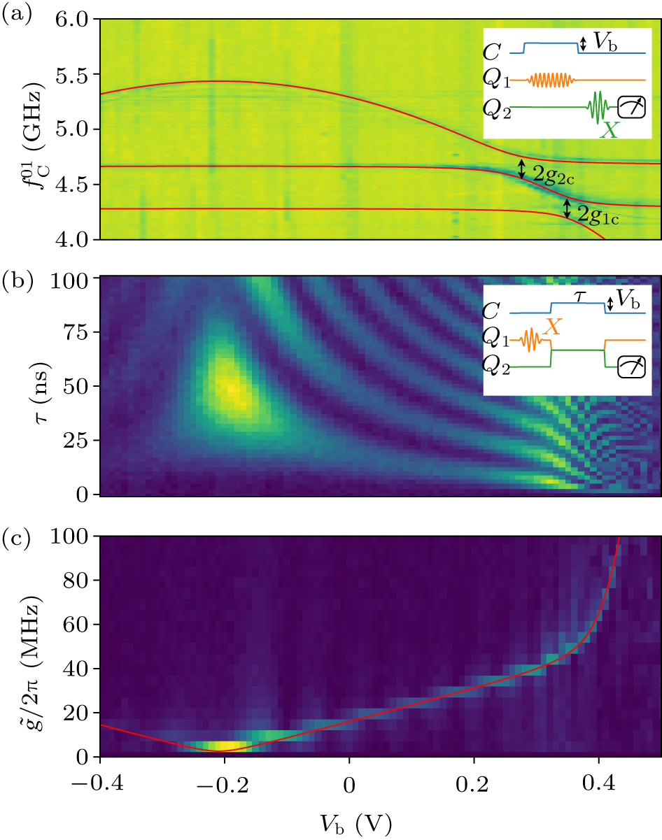
In the present work, we investigate adiabatic and diabatic CZ gates in two Xmon qubits coupled with a tunable coupler system, as shown schematically in Figs. 1(a) and 1(b). Each qubit is capacitively coupled with a coupler which can be seen as an Xmon qubit. Two qubits are also directly coupled via the capacitance. The Hamiltonian of the system can be written as^[24]1H/ℏ=∑i=1,2,cωiai+ai+αi2ai+ai+aiai+∑i≠jgij(ai+aj+aiaj+),where ω_i(i = 1,2,c) are the frequencies of the qubits (Q₁, Q₂) and the coupler (C), ai+ and a_i (i = 1,2, c) are creation and annihilation operators of Q₁, Q₂, and C, respectively. g_1c (g_2c) is the coupling strength between C and Q₁ (Q₂) and g₁₂ is the direct coupling strength between Q₁ and Q₂. The maximum frequencies of Q₁, Q₂, and C are ω1max/2π=4.508 GHz, ω2max/2π=4.701 GHz, and ωcmax/2π=5.419 GHz; and the anharmonicities are α₁/2π = –290 MHz, α₂/2π = –306 MHz, and α_c/2π = –124 MHz, respectively. The effective coupling strength^[2,24] between Q₁ and Q₂ is2g∼≈g1cg2c2(1Δ1c+1Δ2c)+g12,where Δ_ic = ω_i – ω_c (i = 1,2). In the experiments, the value of g_1c(g_2c) can be extracted from the spectrum of qubits or coupler. Figure 2(a) is the spectrum of coupler C. Since coupler C does not have the readout resonator, we use a novel method indicated in the inset of Fig. 2(a). The coupler C could be driven by a microwave pulse through the XY control line of Q₁. If the microwave resonates with coupler C which is excited from |0〉 to |1〉, the frequency of Q₂ will shift due to Lamb shift. Therefore, when applying a π-pulse on qubit Q₂, the population of excited state Q₂ will be decreased. The frequency of the coupler C coupled with qubits Q₁ and Q₂ versus the amplitude of the bias pulse (V_b) of the coupler C is shown in Fig. 2(a). The anti-crossing shows that the coupling strength g_1c/2π(g_2c/2π) is ∼ 100 MHz. The direct coupling strength value g₁₂ can be derived from g∼ which can be extracted from iSWAP experiment. As indicated by the inset of Fig. 2(c), setting up the frequencies of Q₁ and Q₂ on resonance (4.110 GHz) and then sweeping the amplitude V_b and duration time τ of the bias pulse, a chevron pattern of iSWAP experiments can be measured, as shown in Fig. 2(b). The spectrum of two-qubit coupling strengths can be obtained by the Fourier transform of iSWAP time traces as shown in Fig. 2(c) and the light line in Fig. 2(c) indicates that the coupling strength g∼/2π can be changed from 0.4 MHz to 80 MHz by adjusting the frequency of coupler C. Substituting V_b, g∼ and frequencies of Q₁, Q₂ and C into Eq. (2), we can obtain the direct coupling strength of Q₁(Q₂), g₁₂/2π = 5 MHz.

View original graphic| Download| PPT slide

Fig. 1.   (a) and (b) The schematic electrical circuit and optical micrograph of three Xmon qubits (Q₁, Q₂ and C). Q₁ and Q₂ are used as the computational qubits with XY and Z control and coupled with the λ/4 resonators R₁ and R₂ for quantum state readout. Qubit C can be seen as the tunable coupler (C) with only the Z control.

View original graphic| Download| PPT slide

Fig. 2.   (a) The frequency of the coupler C coupled with qubits Q₁ and Q₂ versus the amplitude of the bias pulse (V_b) of the coupler C. The inset is the schematic diagram. The red curves are numerical simulation results fitting the spectrum of qubit–coupler–qubit systems. Two double arrow segments indicate the anti-crossing points and the coupling strength g_1c/2π = g_2c/2π = 100 MHz. (b) The iSWAP oscillation when changing the amplitude V_b of the bias pulse of the coupler C. The inset is the schematic of iSWAP experiment. (c) Fourier transform of iSWAP oscillation in (b). The effective coupling strength \stackrel{\sim }{g}/2\pi can vary from 0.40 MHz to 80 MHz. The red curve shows the calculated results with g₁₂/2π = 5 MHz.

Results and discussion

To easily understand how to operate the qubit–coupler–qubit systems, we use |Q₁,C,Q₂〉 to describe the energy-eigenstates. When performing CZ gates, the computational state |101〉 should be an adiabatic evolution from the idle points close to the region where |101〉 has coupling with another non-computational state (such as |011〉 or |200〉),^[yan18] then back to the idling points with no leakage to these non-computational states. Thus the state |101〉 will accumulate a conditional phase. In order to satisfy adiabatic evolution, the gate time should be greater than 1/g_1c to make sure that there is no leakage to another non-computational state. In our experiment, we firstly bias the Q₁, Q₂, and C at the frequencies of fQ101=4.283 GHz, fQ201=4.679 GHz, and fc01=5.419 GHz, respectively, as idling points where the effective ZZ interaction coupling is smaller than 500 kHz and the two qubits have better coherence time (the T₁ time is 20.9 μs for Q₁, and 28.8 μs for Q₂). The average single-qubit gate fidelities of Q₁ and Q₂ are 99.6% and 99.7%, respectively. Since Q₁ and Q₂ have strong coupling strengths with C, a half-period cosine shape pulse with duration time of 30 ns will satisfy the adiabatic evolution condition.

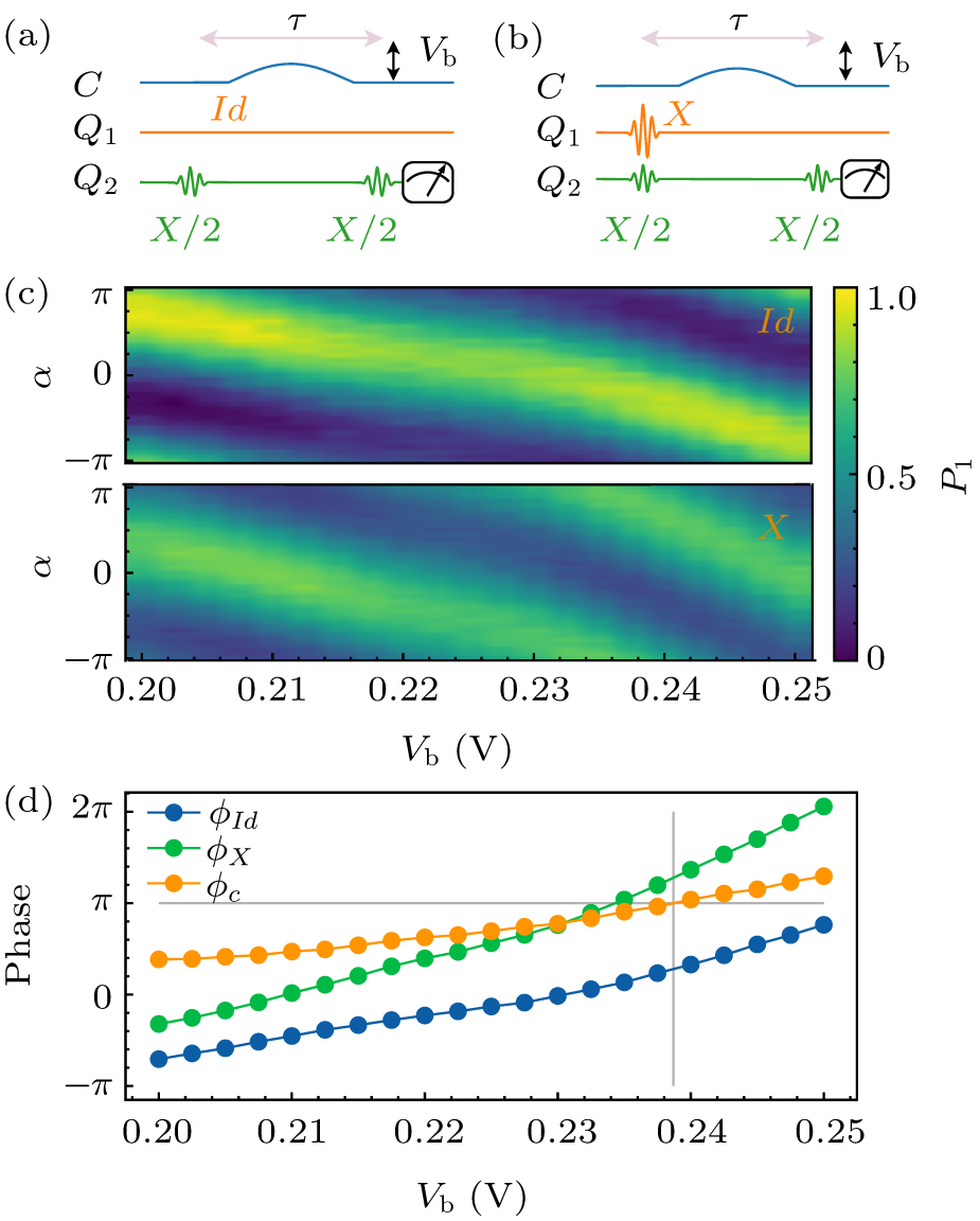
To calibrate the conditional phase, the Ramsey-type experiments are performed as shown in Fig. 3. Figures 3(a) and 3(b) are the control pulse sequence and the qubit Q₁ is prepared in the ground state |0〉 and excited state |1〉, respectively. Figure 3(c) shows the Ramsey oscillation results of qubit Q₂ versus the second X/2 gate phase degree α with different amplitude V_b of coulper C flux pulse. The top and bottom panels correspond to Q₁ initialized in the ground and excited states, respectively. The initial phases ϕ_Id and ϕ_X can be extracted by fitting the Ramsey oscillation trace. Then we can get the relationship between the conditional phase ϕ_c = ϕ_X – ϕ_Id and V_b. As shown in Fig. 3(c), the yellow line corresponds to ϕ_c versus V_b. We can use V_b = 0.2382 V to get the conditional phase ϕ_c = π. ϕ_Id is a local dynamical phase accumulated on Q₂ which can be easily compensated by a virtual Z gate.^[mcka2017] By exchanging the roles of Q₁ and Q₂ in the same experiment, the local phase on Q₁ can also be measured.

View original graphic| Download| PPT slide

Fig. 3.   (a) and (b) Schematic of a Ramsey-type experiment measuring the conditional phase of CZ gate. Qubit Q₁ is prepared in its ground or excited state. Two π/2-pulses (the second π/2-pulse has a phase shift α) are applied on qubit Q₂ with an interleaved idle gate of duration τ, during which the CZ gate (an half-period cosine shape pulse) is applied on coupler C. (c) The oscillations of the population of qubit Q₂ are measured by sweeping the amplitude V_b of CZ gate and the second X/2 gate phase shift α. The top and bottom figures are Q₁ in its ground state and its excited state, respectively. (d) The initial phases ϕ_Id and ϕ_X of the oscillation traces in (c) are fitted as a function of V_b, which are displayed by the blue and green lines, respectively. The conditional phase ϕ_c = ϕ_X – ϕ_Id can be extracted as a function of V_b (yellow line). The gray criss-cross line indicates ϕ_c = ϕ with proper V_b.

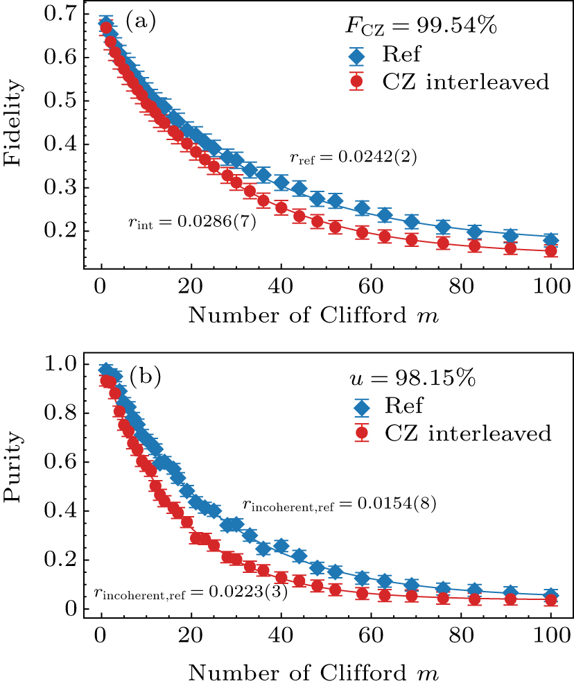
The Clifford based randomized benchmarking (RB) method can be used to assess and optimize the performance of adiabatic CZ gates,^[8,37–41] which is performed by applying a gate sequence of m two-qubit Clifford gates followed by an additional (m + 1)th gate to invert the whole sequence. Figure 4(a) shows the sequence fidelity as a function of m for both the reference and CZ-interleaved cases. The results are the average of 100 random samples. The parameters of adiabatic CZ gate are obtained by implementing Nelder–Mead (NM) optimization algorithm in 100 evaluations. We can obtain the decay constants p_ref and p_int from fitting with the exponential function F = Ap^m + B, and then the error rate per Clifford gate r_ref and r_int from r = 3/4 (1 – p). The CZ gate error rate can be extracted from r_CZ = 3/4(1 – p_int/p_ref) and the CZ gate fidelity from F_CZ = 1 – r_CZ. The average error rate per Clifford gate of our scheme is r_ref = 0.0242(2), and r_int = 0.0286(7) for interleaved, as shown in Fig. 4(a). The CZ gate error r_CZ = 0.0046(2). The fidelity of adiabatic CZ gate is F_CZ = 99.53(8)%. To estimate the decoherence error, we also measure the two-qubit purity benchmarking (PB)^[42,43] as shown in Fig. 4(b). We use the exponential function F = A’u^{m – 1} + B’ to fit sequence purity as a function of m, and obtain the purity error rate from rincoherent=3/4(1−u). The average purity error per Clifford gate is r_{incoherent, int} = 0.0223(3). The average purity error of interleaved sequence is r_{incoherent, ref} = 0.0154(8). As a result, we estimate the incoherence error contribution to be r_{incoherent, ref}/r_ref = 64% of the total errors per two-qubit gate.

View original graphic| Download| PPT slide

Fig. 4.   Fidelity and error analysis of the adiabatic CZ gate. (a) Measured sequence fidelity (100 averages) as a function of the number of Cliffords m for both the reference (diamond) and interleaved (circular) RB experiments. Error bars are the standard deviations from the mean. (b) Measured sequence purity (100 averages) as a function of the number of Cliffords m for both the reference (diamond) and interleaved (circular) PB experiments.

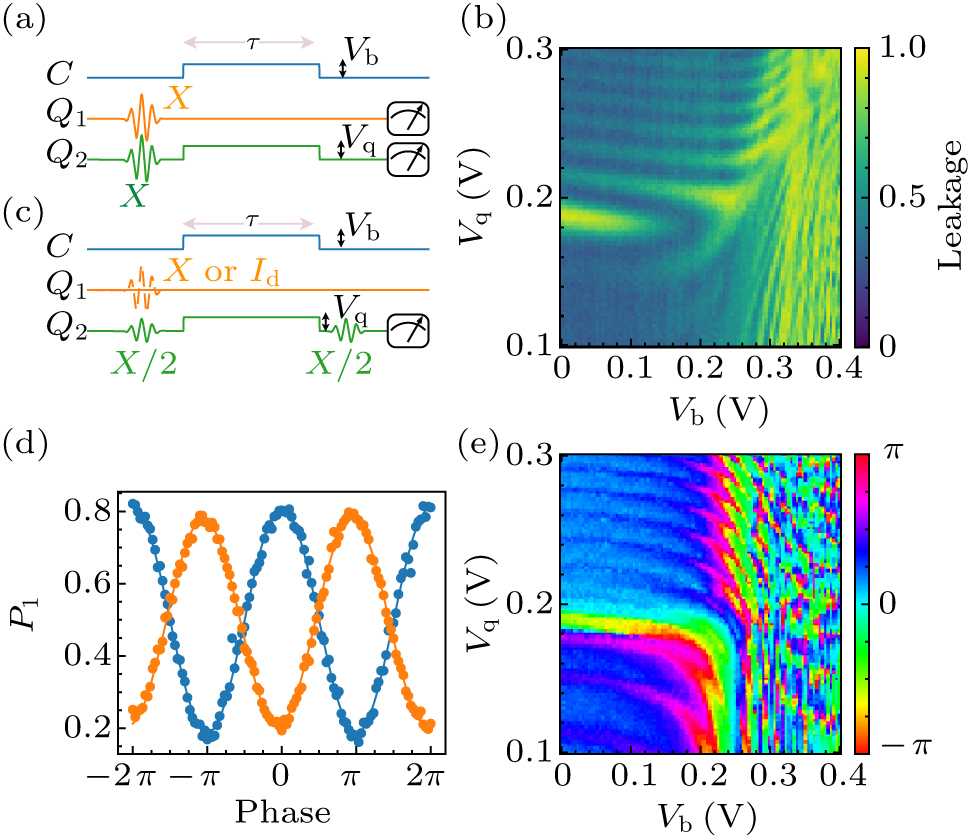
To realize a faster CZ gate, the two-qubit gates need to have a stronger effective coupling strength g∼. From Fig. 2(c), the maximum of g∼ is up to 80 MHz. So we can choose τ ≈ 18 ns as the duration time of CZ gate. However, the evolution of CZ gate will not satisfy adiabatic conditions, which will induce the leakage error. To simplify diabatic CZ gate operation, the square-shaped pulse is used with distortion correction.^[Rol19] Here we have two main controllable parameters, the coupling g∼ and frequency detuning Δ=fQ201−fQ101 to realize the diabatic CZ gates. To adjust Δ value in experiments, we fix Q₁ frequency at the idle points and change the flux bias pulse amplitude V_q of Q₂. Before calibrating the conditional phase, we should exactly identify the leakage versus coupling strength g∼ and frequency detuning Δ. As shown in Fig. 5(a), we initialize two qubits in the excited state and then perform the diabatic CZ gate. If leakage occurs, the population of the ground state of the lower frequency qubit will increase. By sweeping the voltage of V_b and V_q, we can map out leakage errors. The result is shown in Fig. 5(b), where the dark region means the low-leakage errors. After calibrating the conditional phase by executing Ramsey-type experiments, we can get the relationships between ϕ_c and V_b, V_q. Figure 5(c) shows the experimental control pulse sequence which is similar to the adiabatic CZ gates except that the square-shaped pulse is applied and the values of Q₂ flux bias pulse amplitude V_q are explored. The measurement result is shown in Fig. 5(e). The red regions correspond to ϕ_c close to π or –π. As a result, we can pick up appropriate V_b and V_q values to satisfy ϕ_c = π, then check leakage errors in Fig. 5(b). We find that V_b = 0.173 V and V_q = 0.174 V satisfy both constraint conditions. Figure 5(d) shows the results of the qubit Q₂ Ramsey oscillations under these conditions. The phase difference of the two oscillations is π, which means the conditional phase ϕ_c = π.

View original graphic| Download| PPT slide

Fig. 5.   (a) The control sequence to measure leakage errors when implentmenting the diabatic CZ gates. (b) Leakage error results after CZ gates. (c) Schematic of a Ramsey-type experiment measuring the conditional phase of diabatic CZ gates. The pulse shape of diabatic CZ gates is a square-shaped pulse of duration τ = 18 ns. Qubit Q₁ is prepared in its ground or excited state. (d) The results of the Ramsey oscillations under V_b = 0.173 V and V_q = 0.174 V. The conditional phase ϕ_c = π. (e) The conditional phase results after CZ gates.

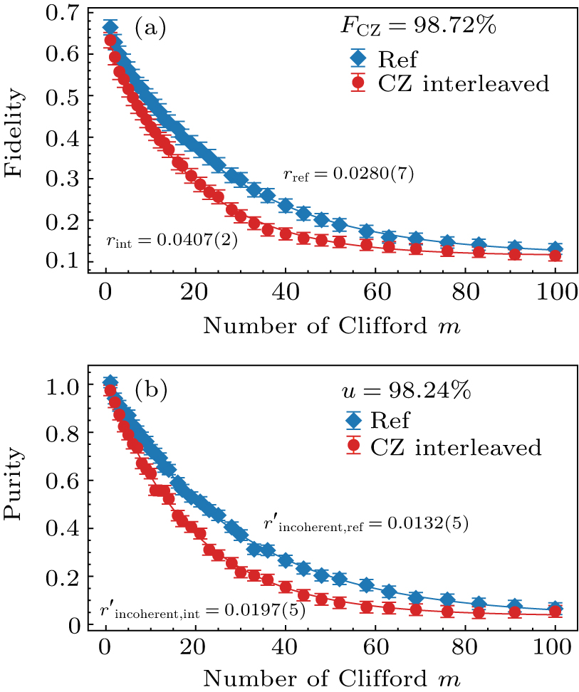
Then RB is used to optimize the fidelity of CZ gate by NM algorithm. The best optimization result is shown in Fig. 6(a). The optimized CZ gate time is 19 ns. The average error rate per Clifford gate r′ref=0.0280(7) and r′int=0.0407(2). The CZ gate error rate r′CZ=0.0127(8). The fidelity of diabatic CZ gate is F_CZ = 98.72(2)%. As shown in Fig. 6(b), the sequence purity r′incoherent,int and r′incoherent,ref are 0.0197(5) and 0.0132(5), respectively. The incoherence error contributes about 47% of the total errors per two-qubit gate.

View original graphic| Download| PPT slide

Fig. 6.   Fidelity and error analysis of the diabatic CZ gate. (a) Measured sequence fidelity (100 averages) as a function of the number of Cliffords m for both the reference (blue) and interleaved (red) RB experiments. Error bars are the standard deviations from the mean. (b) Measured sequence purity (100 averages) as a function of the number of Cliffords m for both the reference (green) and interleaved (yellow) PB experiments.

Conclusion

In summary, we experimentally constructed a tunable-coupled two-qubit system, and realized high fidelity CZ gate in two different schemes. The highest RB fidelities of the adiabatic and diabatic CZ gates we achieved were 99.53(8)% and 98.72(2)%, respectively. The adiabatic CZ gate defined by a cosine flux pulse on coupler required fewer calibrations compared to diabatic CZ gate, which was implemented by applying parallel square-sharped flux pulses both on coupler and one of the frequency tunable qubits. Purity benchmarking which describes incoherence error was also studied. We found that incoherence error contributed 64% and 47% in total error per Clifford gate for adiabatic or diabatic CZ gates, respectively.

Reference

View Option

• By original order
• By published year
• By cited within times
• By Impact factor