


Chaotic signal denoising algorithm based on sparse decomposition
Cite this Article
Huang Jin-Wang, Lv Shan-Xiang, Zhang Zu-Sheng, Yuan Hua-Qiang. Chaotic signal denoising algorithm based on sparse decomposition. Chinese Physics B, 2020, 29(6): 060505 
Permissions
Chaotic signal denoising algorithm based on sparse decomposition
† Corresponding author. E-mail:
Project supported by the National Natural Science Foundation of China (Grant No. 61872083) and the Natural Science Foundation of Guangdong Province, China (Grant Nos. 2017A030310659 and 2019A1515011123).
Abstract
Denoising of chaotic signal is a challenge work due to its wide-band and noise-like characteristics. The algorithm should make the denoised signal have a high signal to noise ratio and retain the chaotic characteristics. We propose a denoising method of chaotic signals based on sparse decomposition and K-singular value decomposition (K-SVD) optimization. The observed signal is divided into segments and decomposed sparsely. The over-complete atomic library is constructed according to the differential equation of chaotic signals. The orthogonal matching pursuit algorithm is used to search the optimal matching atom. The atoms and coefficients are further processed to obtain the globally optimal atoms and coefficients by K-SVD. The simulation results show that the denoised signals have a higher signal to noise ratio and better preserve the chaotic characteristics.
1. Introduction
Chaos phenomenon widely exists in astronomy, meteorology, stock, and so on.[1,2] Some chaotic system can be described by definite equations, but its behavior is similar to stochastic and has the characteristics of broadband and similar to noise.[3,4] Because of the measurement accuracy and external influence, the actually measured chaotic signal is inevitably mixed with noise. Therefore, the characteristics of chaotic signals may be concealed, affecting the accuracy of parameter calculation and prediction of the signals, so the research of chaotic signal denoising algorithm is very important. And the non-linearity and broadband characteristics of chaotic signals makes the denoising more challenging.
The current denoising algorithms for chaotic signals can be classified into three categories. One is that the system model and parameters are known. The recursive expressions of chaotic signals are used as state equations, the adaptive filter, such as unscented Kalman filtering and cubature Kalman filter, is adopted to estimate the signal.[5–7] These methods can achieve online denoising, but the system model and parameters need to be known as a prior. The second is that the system model is known but the parameters are unknown. The phase space denoising method proposed in Ref. [8] belongs to this kind, which explicitly uses the source expression of the chaotic signals, but the recursive parameters are estimated by a least square method in the algorithm. Finally, the global error of the estimated signal is minimized. The third is that the system model and parameters are unknown. These algorithms belong to a completely blind. Wavelet threshold (WT) algorithm,[9,10] local curve fitting (LCF) algorithm,[11,12] and empirical mode decomposition (EMD) algorithm[13,14] are representative in all-blind methods. Essentially, they make use of the low-frequency property of chaotic flow signals, and carry out low-pass filtering while preserving the non-periodic property as far as possible in the filtering process. Their validity depends on the determination of the filtering boundary. The WT algorithm sets the coefficients to zero (hard threshold) under a certain threshold in high frequency band. The LCF algorithm performs hard projection under an optimal window length. The key of the EMD algorithm is to select the optimal number of eigenfunctions to reconstruct the source signal.
Based on these existing algorithms, we propose a noise suppression algorithm using sparse decomposition[15,16] and K-SVD.[17] Since the decomposition coefficient of noise in the dictionary is not sparse, the non-zero coefficients cover the whole transformation domain and generally are small compared with the coefficient of the signal. Moreover, the sparse decomposition coefficient of the signal in the dictionary is sparse, only K non-zero coefficients exist, the coefficient of the noisy signal has only K big coefficients. By decomposing the noisy signal in the dictionary A and selecting only the first K big coefficients, the linear combination of the atoms corresponding to these K large coefficients can approximate the clean signal. The approximation signal obtained contains most of the information of the useful signal and discards most of the noise information, which achieves the purpose of noise elimination.
The innovation of this algorithm lies in using noise intensity to dynamically determine the sparsity of the reconstructed signals, giving a low-complexity dictionary design scheme and optimizing by the K-SVD algorithm. The organizational structure of this paper is as follows: The second part introduces the sparse decomposition denoising model, the third part introduces the algorithm and describes the principle of each step in detail, and the fourth part analyzes the algorithm. The fifth part compares the algorithm with other classical algorithms through numerical simulation, and finally comes to the conclusion.
2. Signal model


The observed noisy signal y(n) from a noise-free signal x(n) can be modeled as

As the signal is divided into segments and processed, we use the window function F(y(n),M′) with window length M′ = 2M + 1 for signal segmentation, y(n) is segmented with length M′ and the moving step is M each time. The signal model can be rewrite in vector form yt = xt + vt. Here yt = [y(t),y(t + 1),…,y(t + M′ – 1)]T ∈ ℝM′, xt and vt have the similar expression. All the vectors yt form a matrix Y = [y1, y2, …, yL], where L = N/M and Y ∈ ℝM′ × L.
For the noisy observed signal yt, the sparsest representation is then the solution to the optimization problem[15]

Usually the problem (P0,δ) demands exorbitant computational efforts in general and does not have a unique sparse solution. If (P0,δ) has the sparsest solution, the corresponding expression can be solved. In the case of noise, we can pursue a strategy of convexification, replacing the ℓ0-norm in Eq. (


3. The proposed denoising algorithm
By decomposing the contaminated signal and selecting only the first K large coefficients, the linear combination of these K large coefficients and the corresponding atoms can approach the clean signal and the purpose of noise cancellation can be achieved. Since selecting the sparsity of each frame, setting up a suitable dictionary A and optimizing the atoms and coefficients are the key parts of this denoising algorithm, we propose a dynamic determination of sparsity, using the iterative equation expansion of the signal to get the dictionary and K-SVD algorithm to optimize the atoms and coefficients here. Figure
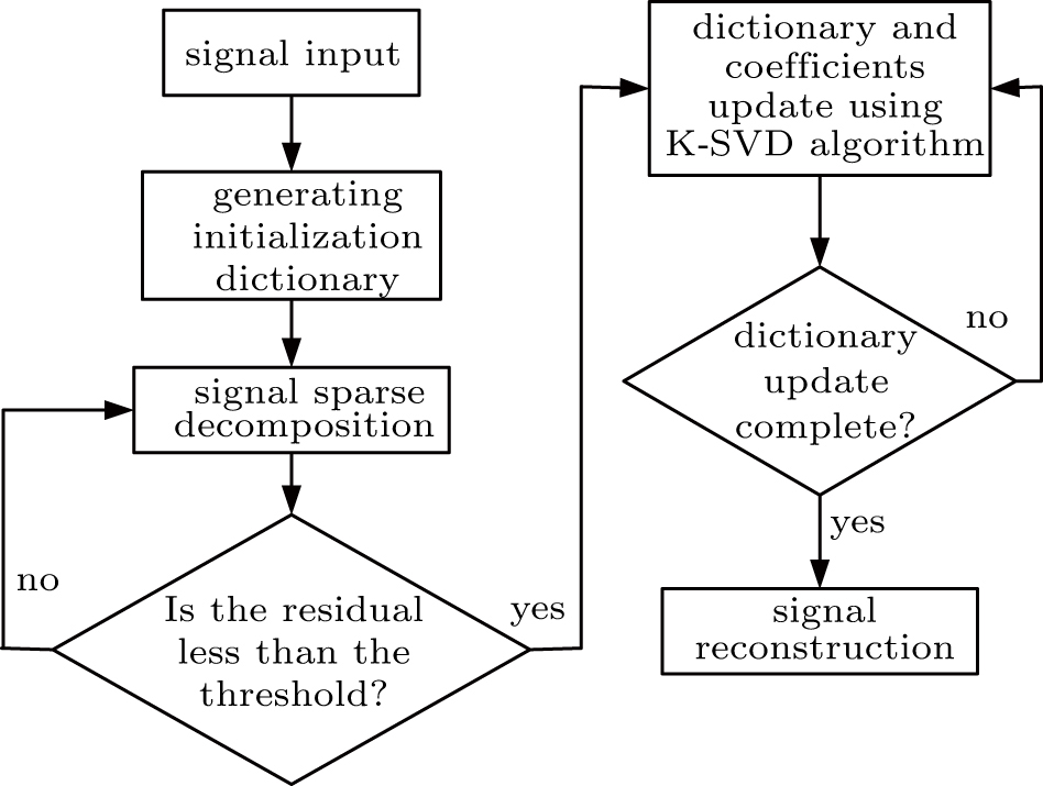 | Fig. 1. Block diagram of sparse decomposition based denoising algorithm. |
3.1. Sparsity determination


The energy of noise can be roughly estimated by means of least total variation or least-squares principle in the case of blind processing,[22,23] the sparsity in the denoising model is based on the parameter of noise intensity. Define the problem

3.2. Dictionary construction

The chaotic flow signal can be described by differential equation 


3.3. Signal sparse decomposition
For the problem 
The initial residual R1 = yt, is the original signal, the orthogonal set of selected atoms is D = dp,p = 1,2,…,k, and the atoms are selected according to certain principles in the iterative process to ensure the minimum residual between the sparse representation result and the original signal.
(1) Select the atom corresponding to the maximum result of residual and inner product in turn,

(2) The above atoms are orthogonalized by Schmidt orthogonalization method,
(3) Normalize dm,

(4) Projecting the residual component Rm onto dm,

3.4. Dictionary update


All the selected atoms are updated one by one using the K-SVD algorithm for global optimum. The atoms and the corresponding coefficients are updated simultaneously.
Choose a column dk (i.e., the k-th atom) in the dictionary and the k-th row of the coefficient matrix S corresponding to dk, which is recorded as 


Define ωk as the indicator set that points to the atom dk in sample yt, namely, the non-zero position in 


Error matrix 

We update all the atoms in the atomic set D sequentially from the first column to the last column, and the optimized dictionary 


3.5. Signal recovery
The sparse coefficients and optimized dictionary are obtained by sparse decomposition of y = [y1, y2, …, yL] after steps 3 and 4. We obtain the reconstructed signal 
4. Algorithm analysis
Based on the matrix A, the received signal can be rewritten as y = As + v when the subscript is omitted. We discuss why the number of selected atoms in A is reduced when the noise increases. In OMP algorithm, the residual of the k-th step can be expressed as[20]

According to the analysis of OMP algorithm in Ref. [20], if the real support set of pure data projected to A is recorded as AΓ, then the definition of maximum inner product coefficient can be derived from qk and vk in Eq. (


In assessing complexities, the algorithm is composed of iterating on three main stages: sparse coding (OMP process), dictionary update, and final averaging process. As mentioned in Ref. [29], both stages can be done efficiently in O(JM′kLnz) per segment, where J is the number of iterations in updating dictionary, M′ is the size of the segment, k is the number of atoms in the dictionary, and Lnz is the maximal number of non-zero elements in each coefficient vector.
5. Simulation
The denoising of chaotic signals should not only be reflected in the improvement of SNR, but also in the maximum restoration of the characteristic parameters of the chaotic signals. In this section, the sparse decomposition based denoising (SDD) algorithm is compared with WT algorithm, LCF algorithm, and EMD algorithm from the aspect of SNR improvement, root mean square error (RMSE), and phase diagram recovery. The nonlinear time series data are generated from the following Lorenz system equations:[26]


Figure
 | Fig. 2. (a) SNR improvement and (b) RMSE of different denoising algorithms under different noise intensities. |
In order to reflect these differences more intuitively, figure
 | Fig. 3. Comparison of the reconstructed attractors by different denoising algorithms: (a) the original pure data, (b) the signal after noise pollution, and (c)–(f) the signal recovered by SDD, WT, LCF, and EMD, respectively. |
The proliferation exponent (PE)[27] is used here to analyze the chaotic characteristics of the reconstructed signal. Although the Lyapunov exponent (LE)[28] can better reflect the chaotic properties of signals from the definition of chaos, its calculation method for continuous chaotic signals is based on the Jacobian matrix of the definition, which is not suitable for the calculation of a large number of sample data. The proliferation exponent can largely reflect the chaos characteristics of the original signal when the input sample data is large enough. The proliferation exponent is defined as

Here we use a Lorenz signal with length of 8000 and sampling interval of 0.05, the same simulation parameter settings as the above. In terms of selecting the value of control factor α, it should be noted that since the selection of α takes the sampling step into account, that is, the optimal α value is set based on the sampling step to best reflect the chaotic characteristic. The simulation results with different α values may be slightly different. Here we set α = 6 and calculate the PE of the restored signal by different algorithms. As shown in Fig.
 | Fig. 4. Comparison of proliferation exponents of the restored signal by different denoising algorithms. |
6. Conclusion
Based on the theory of sparse decomposition and K-SVD, we propose a chaotic signal denoising algorithm with dynamic sparsity determination, dictionary constructed by signal iteration equation and K-SVD optimization. The special point of this algorithm is that the constructed dictionary over complete projection matrix has sufficient frequency-domain components, so that it can better represent each segment of the signal. The K-SVD optimization process further improves the noise reduction. The simulation results show that the algorithm has better SNR improvement and RMSE than the other three denoising algorithms, especially in the case of low SNR. For the PE value calculation which characterizes the chaotic signal, the algorithm in this paper has better performance than the other three denoising algorithms.
Reference