The key to studying time series from the perspective of complex network theory is to choose an effective conversion method. As mentioned before, Zhao et al. presented a practical transformation approach between time series and complex networks based on the amplitude difference of data points.^[16] Let {p_t |t = 1,2,…,N} be a scalar time series of N observations and ε be a threshold. The adjacency matrix of the transformed network is defined as A = {a_st |s = 1,2,…,N; t = 1,2,…,N}, where a_st = 1 if |p_s − p_t| < ε, otherwise a_st = 0. That is, there exists a link from node s to node t if the distance between the nodes is less than the threshold. The basis of the equivalence theorem of dual characterization between time series and complex networks is the topological homeomorphism theorem and quasi-isometric theorem. They found that the waveform of the reconstructed time series and the original time series are exactly the same, which means that this conversion method implements an equivalently mathematical description of time series under network representation.

Suppose that there is only one financial asset in the stock market. The market consists of I heterogeneous active traders who take long position or short position in this security. The movement from the (t − 1)-th to the t-th Walrasian equilibrium is driven due to the arrival of new information. Let P_t denote the current market price, and P_ti the i-th trader’s reservation price which is his belief about the stock price in the future at time t, where i = 1,2,…,I. Assume that there are no transaction costs and the I traders differ only in their beliefs (Since different traders only differ in their beliefs, we only study the investment behavior of the i-th active trader for convenience), then the inter-trader differences in their beliefs will arise from different expectations about the future and from different needs to transfer risk through the market.

Consequently, all price risk is viewed as falling on terminal wealth. The agent is assumed to choose position Q_ti to maximize the expected utility of terminal wealth. The gain attributable to this speculative position and hence its contribution to terminal wealth is

Equilibrium requires , which indicates that the weighted average of the reservation prices

Now, we consider the movement from the (t − 1)-th to the t-th equilibrium. A piece of news arrives at the market and changes the individuals’ reservation prices. Since in equilibrium, the total number of buy orders matches the total number of sell orders, we have

The resulting change in the market price is the weighted average of the increments with respect to the traders’ reservation prices, which implies

We have introduced the decision-making behavior of rational investors above, where market prices and investor’s reservation prices are both exogenous. However, we know that investors cannot be rational all the time in real life, so their investment decisions may be affected by their sentiment. For example, if the market trend is particularly apparent, the trader will be sure of his belief, and hence increasing his positions. That is what we see as the “buying the winners” strategy. Moreover, a trader will become more optimistic when he tends to judge correctly for the market price changes recently or after a high level of return,^[42] which will lead to excessive transactions.

We can see that investors’ seemingly opposite behaviors, such as following others and believing in themselves, can both lead their desired positions to increase. This raises the question whether an investor can behave both herding and confidence at the same time. If so, does any connection exist between them? Moreover, what is their combined effect on the investor’s position? To answer these questions, we construct a market network that represents the market trend and an investor network that represents the past judgments from the perspective of a representative investor in the following subsection.

Following the work of Zhao et al.,^[16] we will build complex networks based on the time series of price changes (Due to the relatively large fluctuations in the time series of stock prices, which will interfere with the study of statistical properties of the data, used in this paper are the differenced stock prices, that is, the time series of price changes) and past judgments for the representative i-th investor.

Firstly, in the market network, we define node t as the market price change at time t and the edge from node (t − m) to node t as the influence of the market price change at time (t − m) on the market price change at time t. Considering that the current market price change cannot have an influence on the past market price changes, and the memory length of the trader is limited (assuming the i-th investor’s memory length is M) (Although each one observes the same market prices, their herding behavior may be different due to the various memory lengths), we give definitions below.

Similarly, we can construct an investor network based on the past judgments of the i-th investor.

Every time when a piece of new information arrives at the market, each trader will update his reservation price and then obtain the market clearing price. If the directions of the two price changes are the same, the trader will make the right investment decision because his judgment is consistent with the judgment of the majority. Therefore, for the investor network, we employ node t to represent the product of the market price change and the trader’s reservation price change at time t and the edge from node (t − m) to node t to represent the effect of the trader’s judgment at time (t − m) on the judgment at time t. Being the same as the market network, the trader’s current judgment cannot influence the past judgment, and the memory lengths of different traders are different (assuming that the i-th investor’s memory length is M), we give another definition below.

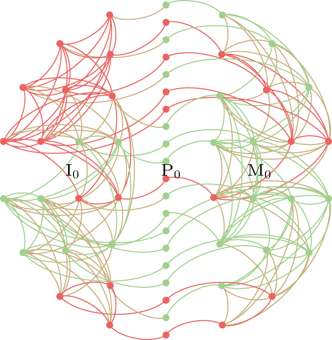
To have an intuitive understanding of the mapping from time series to complex networks, we present the network structures of the stock price series (P₀), the price change series and the investor judgment series together based on the sample of Microsoft’s stock prices during the first 20 trading days in July 2009. Specifically, we transfer the price change series into the market network (M₀) according to Definition 1, which is shown as the right sub-network in Fig. 1. Meanwhile, we map the investor judgment series into the investor network (I₀) by Definition 2 in the left sub-network of Fig. 1. The 20 vertical nodes (P₀) in the center of Fig. 1 correspond to the 20 observations of the stock price series, which are connected to the nodes at the same time point in the market sub-network and investor sub-network, respectively. That is to say, there are 20 nodes in each sub-network. It is supposed that the investor’s memory length is 5 trading days and the threshold is big enough so that each node has 5 directed edges from its previous 5 nodes. The nodes in gray represent the stock prices. The other nodes are in green if their sizes are above 0, otherwise in red. Since we define the edges as the influence of past nodes on future nodes, the color of the edge is the same as that of its leaving node.

Fig. 1.

	Figure Option ViewDownloadNew Window
	Fig. 1. Network mapping of time series of stock prices, price changes, and investor’s past judgments.

The networks constantly evolve as the stock market moves from one equilibrium to the next one. Due to the similar structure between the market network and the investor network, we take the market network for example to explain the dynamic evolution of the network structure in detail.

It is supposed that there are always N nodes in chronological order of a network. When a piece of news arrives at the stock market, we obtain a new market clearing price, thus a new market price change. At this time, we add a new node to this network and meanwhile delete the first node of the network, so there are still N nodes. Since the memory of investors is limited, we assume that only the previous M nodes can affect the t-th node in the eyes of investors. That is, there will be M directed edges from the previous M nodes to the new t-th node. Then, how is the influence of former nodes on the t-th node judged?

Assuming that every time when a node k is added to the network, the investor will compare the size of the k-th node ΔP_k with the sizes of the previous M nodes ΔP_{k − 1}, ΔP_{k − 2}, …, ΔP_{k − M}. If the difference between ΔP_k and ΔP_{k − m} is smallest, then x_k = m, where x is defined as a discrete variable taken on values 1, 2, 舰, M. This means that the (k − m)-th node has the most significant influence on the k-th node. In other words, the status of node k is more likely to be transformed from the status of node (k − m) than the other previous M nodes. Let k traverse from (t − N) to (t − 1), then will represent the number of times for the status of node k to be transformed from the status of node (k − m) for the previous N nodes of node t. Therefore, we can use the frequency of x = m to represent the transition probability from the (t − m)-th node to the t-th node, which can be expressed as

Meanwhile, the i-th investor compares the size of the k-th node ΔP_k ΔP_ki with the sizes of the previous M nodes ΔP_{k − 1} ΔP_{(k − 1)i}, ΔP_{k − 2} ΔP_{(k − 2)i}, …, ΔP_{k − M} ΔP_{(k − M)i} in the investor network. If the difference between ΔP_k ΔP_ki and ΔP_{k − m} ΔP_{(k − m)i} is smallest, then y_k = m, where y is defined as a discrete variable taken on values 1, 2, …, M. Therefore, the transition probability from the the (t − m)-th node to the t-th node in the investor network can be expressed as

The weighted degree is a critical statistical index in the complex network. The higher the weighted in-degree or out-degree of the node, the more critical the node is in the complex network.^[43] We explore the economic implications of weighted in-degree of the market network in this subsection and weighted in-degree of the investor network in the next subsection.

Based on the dynamic evolution process described above, the weighted in-degree of node t in the market network can be expressed as the sum of the influence of nodes which have direct links to node t on node t, that is,

We can see from Eq. (8) that the magnitude of the weighted in-degree is larger when there is a considerable rise or fall with duration increasing. However, if the prices fluctuate, the magnitude of the weighted in-degree will be smaller. Meanwhile, the herding extent of investors has a similar pattern. When the market is in a booming stage, the herding investors will continue to be bullish because individuals holding most positions are bulls. However, in a recession, herding investors will continue to be bearish because individuals holding most positions are bears.^[44] In a word, the herding extent of investors will accelerate if there is an evident market trend.^[45]

Considering the consistency between the size of the weighted in-degree and the investor’s herding degree with the change of market trend, we can use the absolute value of the weighted in-degree to indicate the investor’s herding extent, that is,

At the beginning of each period t, the i-th trader forms his herding degree based on the past market trend. The higher the absolute value of the weighted in-degree, the stronger the investor’s herding degree will be.

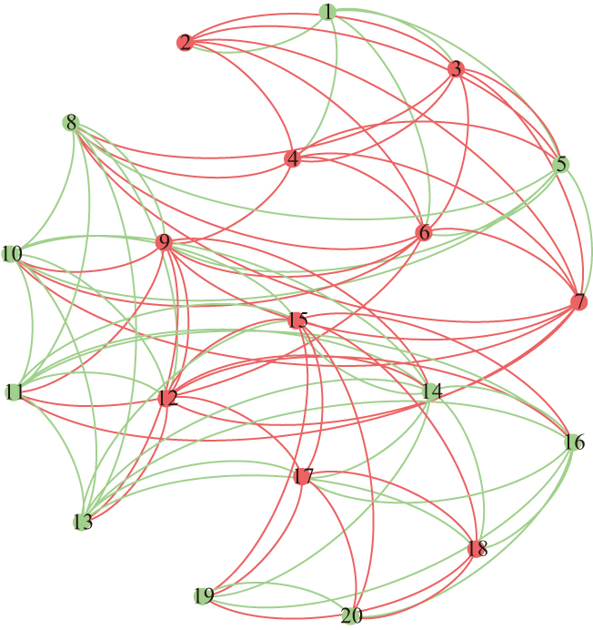
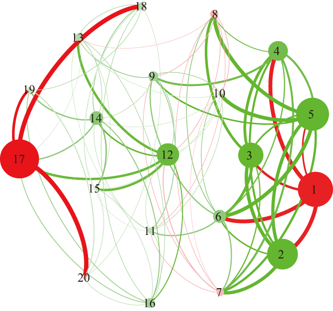
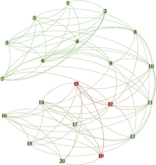
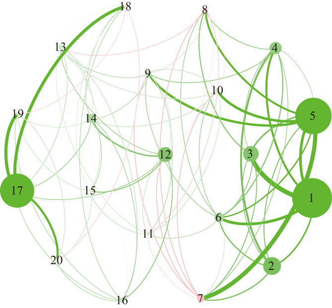
To clearly show the changes of the market network before and after being updated, we construct the market network by using the Microsoft’s transaction data spanning from July 1, 2009 to June 30, 2019 which consists of 2517 observations. Suppose that there are always 20 nodes in a static network, i.e., N = 20, and the memory length of a typical investor is one week, that is, M = 5, then we will update the network by using the method described above. Figure 2 shows the market network before being updated, which is the same as the right half part of Fig. 1, while figure 3 shows the market network after being updated for 10 years. Being the same as Fig. 1, the node is in green if its size is above 0, otherwise in red. The color depth is correlated to the magnitude of the node.

Fig. 2.

	Figure Option ViewDownloadNew Window
	Fig. 2. Market network before being updated.

Fig. 3.

	Figure Option ViewDownloadNew Window
	Fig. 3. Updated market network.

Similarly, we can express the weighted in-degree of node t in the investor network as

If the i-th investor judges correctly at time (t − m), then Δp_{t − m} Δp_{(t − m)i} > 0, otherwise Δp_{t − m} Δp_{(t − m)i} ⩽ 0. The weighted in-degree will increase with the right extent of judgment increasing and decrease with the wrong extent of judgment increasing. Meanwhile, the confidence extent of investors also has a similar change pattern to the weighted in-degree in the investor network. Odean argued that investors’ degree of overconfidence can be measured by their early excess net return.^[37] Many researchers believed that in the stock market, most of investors tended to take too much credit for the excess profits they had obtained, which would produce more trading and volatility.^[30,36,46] In a word, the key to overconfidence is that investors have made the correct judgments many times, and they believe that it is their own abilities that help them make the right judgments. Therefore, we can use the value of the weighted in-degree in the investor network to indicate the confidence extent of investors. At the beginning of each period t, the i-th trader forms his confidence extent based on past judgments. The higher the weighted in-degree, the stronger the investor’s confidence degree will be.

We still use Microsoft’s stock prices to calculate market price changes. However, the data of the traders’ reservation prices are not available, so we simulate the i-th trader’s reservation prices as follows:

Fig. 4.

	Figure Option ViewDownloadNew Window
	Fig. 4. Investor network before being updated.

Fig. 5.

	Figure Option ViewDownloadNew Window
	Fig. 5. Updated investor network.

The common practice of comparing two networks at network level is to compare some main topological indicators, including the network betweenness centralization, network clustering coefficient, and modularity degree.

To verify the generality of the experimental results, apart from employing Microsoft’s transaction data spanning from July 1, 2009 to June 30, 2019 in the previous article, we present the corresponding results of Microsoft’s transaction data from July 1, 2009, respectively, to September 30, 2015, December 31, 2016, and March 31, 2018. We choose different months as the cut-off time so as to exclude the interference of quarterly effects in the stock market. Also, we show the network topological indexes and the correlation coefficients between the node parameter sequences based on the data of the US S&P 500 stock index and the China Hushen 300 stock index. We use M₀ and I₀ to denote the market network and the investor network before being updated, M₁ and I₁ to represent the two networks after being updated. The results are shown in Table 1.

Table 1.

Table 1.

Table 1. Network topological indexes. . Network betweenness centralization Network clustering coefficient Modularity Panel A: Microsoft transaction data spanning from July 1, 2009 to June 30, 2019 M0 0.023 0.382 0.510 I0 0.023 0.382 0.523 M1 0.023 0.382 0.413 I1 0.023 0.382 0.371 Panel B: Microsoft transaction data spanning from July 1, 2009 to September 30, 2015 M1 0.023 0.382 0.362 I1 0.023 0.382 0.351 Panel C: Microsoft transaction data spanning from July 1, 2009 to December 31, 2016 M1 0.023 0.378 0.329 I1 0.023 0.378 0.404 Panel D: Microsoft transaction data spanning from July 1, 2009 to March 31, 2018 M1 0.023 0.382 0.416 I1 0.023 0.382 0.336 Panel E: Hushen 300 transaction data spanning from July 1, 2009 to June 30, 2019 M0 0.023 0.382 0.448 I0 0.023 0.382 0.484 M1 0.023 0.382 0.418 I1 0.023 0.382 0.406 Panel F: S&P 500 transaction data spanning from July 1, 2009 to June 30, 2019 M0 0.023 0.382 0.435 I0 0.023 0.382 0.491 M1 0.023 0.382 0.434 I1 0.023 0.382 0.483

Table 1. Network topological indexes. .

Network betweenness centralization is the average of the ratios of the number of paths that pass through each node to the total number of shortest paths, which can be used to measure the average bridge intermediation of network nodes. Table 1 shows that the values of the network betweenness centralization remain constant after being updated for all the three types of stocks. Besides, the values of the indicator for the market network are the same as those for the investor network at a single point, indicating that the average financial information transfer effects of the two networks are similar to each other.

Network clustering coefficient is a measure of the degree to which the nodes in a graph tend to cluster together. We can see from Table 1 that the value of the network clustering coefficient declines only for the Microsoft data spanning from July 1, 2009 to December 31, 2016. For the three kinds of stocks, the aggregation characteristics in the market network and the investor network are still similar, whether they are updated or not.

Modularity is used to measure the strength of the division of a network into modules that are also called groups, clusters, or communities. Networks with high modularity have dense connections between the nodes within modules but sparse connections between nodes in different modules. From Table 1 it may follow that the values of the modularity of both networks all decline, whether for different updated intervals or classes of stocks. At the same point, there is no much difference in the value between the market network and the investor network.

In this part, we focus on the parameters related to the nodes such as the weighted in-degree, weighted out-degree, and weighted degree (The weighted in-degree in the market network is taken as its absolute value in the following calculation due to its significant economic meaning discussed in Subsection 3.2). The detailed interpretations of each parameter used here are presented as follows.

Weighted in-degree is the sum of the weights of the edges entering a node.

Weighted out-degree is the sum of the weights of the edges leaving a vertex.

Weighted degree is the sum of weighted in-degree and weighted out-degree.

Using the updated networks, we first compute the corresponding parameters of each node. Then, we obtain two parameters series, and thus we can calculate their correlation coefficients. To confirm that the correlation coefficient is only significant between the two networks at the same time, we also calculate the correlation coefficients between the updated market network (M₁) and the investor network before being updated (I₀), and the updated investor network (I₁) and the market network before being updated (M₀) for each node parameter. The results are shown in Table 2.

Table 2.

Table 2.

Table 2. Correlation coefficients for node parameter sequences. . Correlation coefficients Weighted in-degree Weighted out-degree Weighted degree Panel A: Microsoft transaction data spanning from July 1, 2009 to June 30, 2019 M1 ∼ I1 0.662 0.919 0.837 M1 ∼ I0 −0.054 0.243 −0.041 I1 ∼ M0 −0.100 0.040 −0.103 Panel B: Microsoft transaction data spanning from July 1, 2009 to September 30, 2015 M1 ∼ I1 0.602 0.942 0.927 M1 ∼ I0 −0.233 −0.086 −0.359 I1 ∼ M0 −0.096 0.165 −0.105 Panel C: Microsoft transaction data spanning from July 1, 2009 to December 31, 2016 M1 ∼ I1 0.733 0.950 0.957 M1 ∼ I0 −0.355 −0.236 −0.323 I1 ∼ M0 0.122 −0.360 −0.150 Panel D: Microsoft transaction data spanning from July 1, 2009 to March 31, 2018 M1 ∼ I1 0.402 0.746 0.503 M1 ∼ I0 0.556 0.110 0.282 I1 ∼ M0 0.226 −0.066 −0.150 Panel E: Hushen 300 transaction data spanning from July 1, 2009 to June 30, 2019 M1 ∼ I1 0.828 0.958 0.926 M1 ∼ I0 0.182 0.155 0.101 I1 ∼ M0 0.077 0.221 0.250 Panel F: S&P 500 transaction data spanning from July 1, 2009 to June 30, 2019 M1 ∼ I1 0.754 0.922 0.852 M1 ∼ I0 0.118 −0.348 −0.226 I1 ∼ M0 0.078 −0.297 −0.170

Table 2. Correlation coefficients for node parameter sequences. .

From Table 2, we can see that the correlation coefficient of the weighted in-degree series, weighted out-degree series, and weighted degree series between the updated market network and investor network are all around 0.6 in these cases, which indicates a high correlation of the node parameters between the two networks. Correspondingly, we cannot find distinct patterns between the updated market network and the investor network before being updated, nor the updated investor network and the market network before being updated, which further illustrates that the correlation relationship only exists between the market network and the investor network at the same time point.

As demonstrated in Section 3, the weighted in-degrees of the nodes in the market network and the investor network can represent the investor’s herding degree and confidence degree. Due to their critical economic meanings, we focus on the correlation of the weighted in-degree series of the two networks and theoretically derive the conditions for their convergence, which helps us analyze the internal mechanisms behind our conclusions. Then, we obtain

We finish this section by analyzing the internal mechanisms behind our conclusions. We suggest that these two kinds of behaviors that seem to be mutually contradictory are in fact consistent when their variations with the mean of the price changing are low. In particular, when their variations with the market price changing is small, which means that the market price changes are stationary, the market will show a clear trend. According to Eq. (9), the investor’s herding degree will go up because it is easy for him to seize the market trend. Equation (5) shows that the direction of the market price change is the same as that of the reservation price change for most of position holders in the market. Therefore, seizing the market trend means that the investor knows what the majority will do. At this time, it is easy for the investor to make the same decisions as most of position holders do, making him more likely to make the right judgments. Based on Eq. (10), the investor’s confidence degree will increase with the right extent of judgments increasing. Finally, the overconfidence goes up with the accumulation of continuously growing confidence levels. For example, if the price of some stock rises steadily over a period of time, that is, there is a clear upward trend, the investors are more likely to enter into the market or increase their positions, showing herding effects. The herding behavior of investors will push the price to go up further, and investors will obtain positive return, which will enhance their confidence degrees.

However, when the coefficient of variation is large, investors do not have the chance to follow the crowd. At this time, whether investors have made their right judgments is entirely accidental, so a trader’s herding degree is almost not correlated with his confidence degree. For example, if the price of a stock goes up and down like a seesaw for some time, then investors will not have any trends to follow. At this time, some investors will increase their positions, and others will reduce their positions. The irregular behaviors of investors will have an uncertain influence on the direction of price change, so investors cannot continuously obtain positive returns, and their confidence degrees cannot accumulate.