† Corresponding author. E-mail:
Holter usually monitors electrocardiogram (ECG) signals for more than 24 hours to capture short-lived cardiac abnormalities. In view of the large amount of Holter data and the fact that the normal part accounts for the majority, it is reasonable to design an algorithm that can automatically eliminate normal data segments as much as possible without missing any abnormal data segments, and then take the left segments to the doctors or the computer programs for further diagnosis. In this paper, we propose a preliminary abnormal segment screening method for Holter data. Based on long short-term memory (LSTM) networks, the prediction model is established and trained with the normal data of a monitored object. Then, on the basis of kernel density estimation, we learn the distribution law of prediction errors after applying the trained LSTM model to the regular data. Based on these, the preliminary abnormal ECG segment screening analysis is carried out without R wave detection. Experiments on the MIT-BIH arrhythmia database show that, under the condition of ensuring that no abnormal point is missed, 53.89% of normal segments can be effectively obviated. This work can greatly reduce the workload of subsequent further processing.
Arrhythmia manifests as irregularity in heart rate or rhythm, and the exact moment of occurrence is uncertain, usually needing to wear Holter for 24–72 hours to capture. It is time consuming and labor intensive to manually interpret long Holter data by doctors. Therefore, automated analysis is required.
Among the automatic analysis techniques for Holter data, there is a kind of methods which need R wave detection.[1–5] For example, the work[5] separates each heartbeat waveform one by one based on R wave detection, and then sends them to the deep convolutional neural network (CNN) for heart beat classification. The work divides heart beats into one of five categories. This kind of Holter data analysis method starts with the detailed R wave detection that is somewhat hard to accomplish well, which does not conform to the principle from coarse to fine.
A reasonable approach is not to do the R wave detection first, but to make judgments on the electrocardiogram (ECG) data segments, in order that it can screen out normal data segments as many as possible, i.e., reduce the data quantity first on the premise of ensuring the retention of abnormal segments.
Mhuah and Fu[6] divided segments according to whether the distance between ECG segment and nearest non-self match exceeds the threshold. In the method, determining the threshold needs to learn from the abnormal data segment. Acharya et al.[7] proposed to use the deep CNN network to identify four types of ECG segments: atrial flutter, atrial fibrillation, ventricular fibrillation, and normal. Although the shown performance is good, the given classes are too many, needing much more labeled data for training, which means that it is of weak operability and not suitable for preliminary screening.
Chauhan and Vig[8] used the error generated by the LSTM prediction model to classify the segments. If the log(PDF) value of an error exceeds a threshold, the corresponding segment is divided into the anomaly. The threshold is determined as follows: a validation set containing abnormal signals is used, to maximize the F1-score on the validation set to get a fixed threshold, i.e., the target function pursues the largest proportion of true positive samples. However, we think the most important thing in the screening of data is that the abnormal segments cannot be missed. Avoiding false negatives should be the constraint.
The shortcomings of the above screening methods by segment can be summarized as follows: (1) Abnormal segments are needed for learning, which is inconvenient in practice. (2) The design of the objective function is not reasonable, and avoiding false negatives should be the premise to screen away the normal data segments. This paper will propose an improved Holter data anomaly segment screening method based on the LSTM prediction model. It does not need abnormal data for learning. It only needs to monitor the normal ECG signal points for a few minutes to train the prediction model. The determination of the threshold is based on the maximum probability of avoiding missing abnormal data segments.
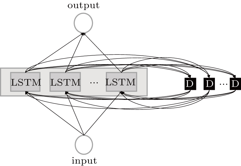
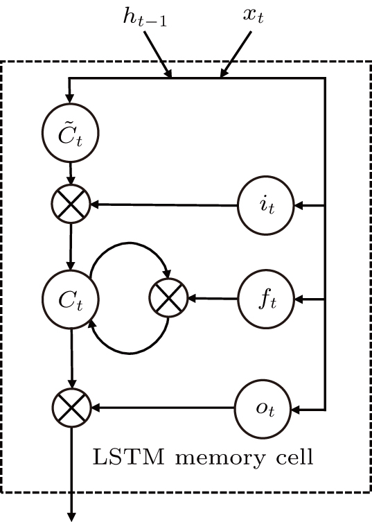
As one kind of RNN networks, the LSTM as shown in Fig.
The input of the input gate [IG] of an LSTM unit is the input vector xt from the previous layer at the current moment and the output vector ht – 1 of all LSTM units of the current layer at the previous moment. After the sigmoid unit (σ(∼)), a real number between 0 and 1 is obtained. Wi and Ui are two weight vectors, and bi is the offset. The forgetting gate [FG] and the output gate [OG] are calculated in a similar manner to the input gate. The unit function for 


The data used in the following study is from the MIT-BIH arrhythmia database.[4] The data in the database was independently labeled by two cardiologists who marked all abnormal beats and added rhythm and signal quality labels. The data for each patient is approximately for 30 min and the sampling rate is 360 Hz, including 2 channels.
In the following study, only 16 patients are selected for modeling research. They are 100, 101, 105, 108, 114, 121, 123, 202, 205, 209, 210, 213, 219, 223, 230, 234. These data have normal sequences which are longer than one minute and can be used for the modeling of this method, while other data does not have long enough normal sequences for this model.
In addition, this study only selects the MLII channel of the 16 data for research. Compared with the other channel, it can better meet the requirements of normal sequences with longer than 1 min.
The whole method consists of two phases: the learn phase and the work phase.
Due to the individual differences between the ECG signals of different patients, each patient data is arranged for their own model learning. In the learn phase, a normal ECG sequence of the patient is required. First pre-process the sequence to reduce noise, and the noise-reduced data is used to train the LSTM network, which is essentially an autoregressive prediction model. Using the trained model, the prediction errors of the input normal data are calculated. On the basis of kernel density estimation (KDE), the probability density function of the prediction errors can be obtained, and subsequently we can determine the prediction error threshold interval for accepting the assumption that the data is normal, as shown in Fig.
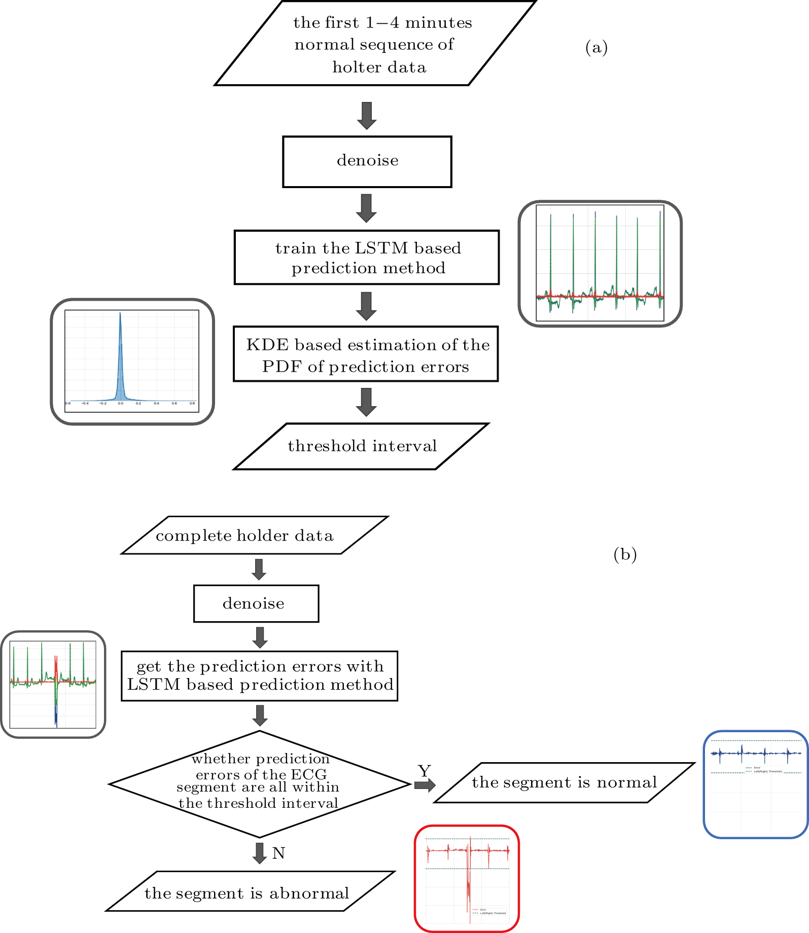 | Fig. 3. Training and working flowchart of the method: (a) the training LSTM model and threshold interval, (b) determining if ECG segment is normal. |
In the work phase, as a judging unit, each ECG segment of a sequence will be classified as a normal one or an abnormal one. The sequence to be tested is sent to the trained LSTM prediction model, and the prediction error of each point in the segment is calculated to see whether any prediction error exceeds the set threshold interval. If yes, it will be an abnormal segment considered. If no, a normal segment considered, which can be screened out. See Fig.
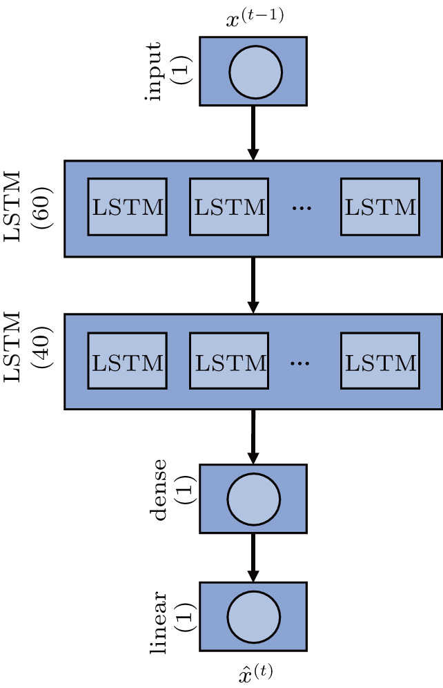
The LSTM network used is called the stacked LSTM network. As shown in Fig.
The cost function L of network training is defined as the mean squared error function (MSE)


Timestep is a parameter that controls the complexity of the training process, and it limits the number of steps where the gradient can expand in the backpropagation. Essentially, it is assumed that the model relies on the current ECG samples and the latest timestep ECG samples.
We define the prediction error e(t) as follows:

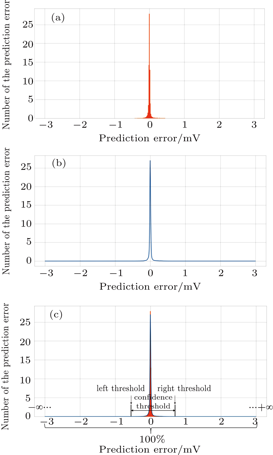
After observing, the histogram of the prediction errors in the experiment, as shown in Fig. 


Set the confidence value α. If a prediction error e(t) in an ECG segment is outside the corresponding threshold interval, the ECG segment can be judged to be abnormal. Since the prediction errors do not obey any classical distribution, it is necessary to calculate the threshold interval by the integration method. According to the known confidence value, the way to obtain the left and right thresholds is as follows: accumulate the probability from the negative infinity to the left threshold γ1 until the sum reaches 1/2(1 – α) and accumulate the probability from the positive infinity to the right threshold γ2 until the sum of the process also reaches 1/2(1 – α), as shown in Fig.
For the data in the selected database, we divide each long sequence into several connected time segments. If there is an abnormal signal point in the time range of a segment, the segment will be marked as an abnormal one; otherwise, it will be marked as the normal. Since a supraventricular ectopic activity[14] has small QRS wave morphological change, the segment with supraventricular ectopic activities is also marked as the normal one in our method. The determination of the length of each segment should make sure the convenience of the doctors observing ECG waveform, and 10 s duration is selected as the size of one segment in this paper. Each patient data is divided into 181 labeled segments.
Each patient’s data is divided into two parts: training set, test set. As shown in Fig.
The ECG data is subjected to discrete wavelet transform (Daubechies 6) for noise and baseline wander removal.[15] Subsequently, to eliminate the problem of amplitude scaling,[16] the sequences are processed via Z-score normalization (

The main objective of the abnormal data screening method proposed in this paper is to eliminate more normal segments to reduce the workload of the subsequent further fine classification, while ensuring that no disease segments are missed. To describe the screening ability for anomalies, we define the evaluation indicator: effective screening rate (ESR).

The condition that FN is 0, means that no abnormal segment is misjudged as the normal. The higher the ESR, the larger the correct rate of the classification result on the normal segments, and the greater the normal segments can be excluded, whereas neither of the abnormal segments can be judged as the normal ones.
The selection of the confidence value needs to be optimized. If the confidence value is set too small, the threshold interval will be too small. This may cause the prediction errors of the normal points to exceed the threshold limit and be misjudged as abnormal. What we need is the maximization of the confidence value under=0 to maximize ESR. After experiments, we find that when the confidence threshold is set to 99.993%, ESR is highest at 53.89%. In other words, 53.89 per cent normal data can be excluded and there is no missed anomaly detection, as shown in Table
| Table 1. Results of all test sets. . |
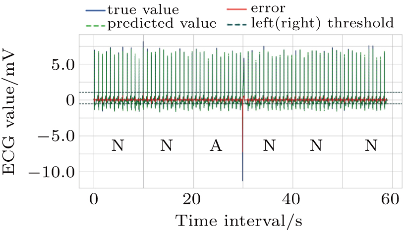
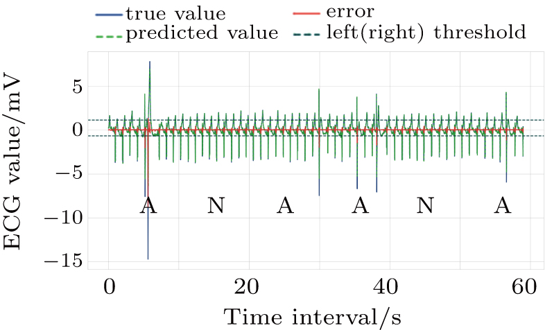
Figures
As shown in Fig.
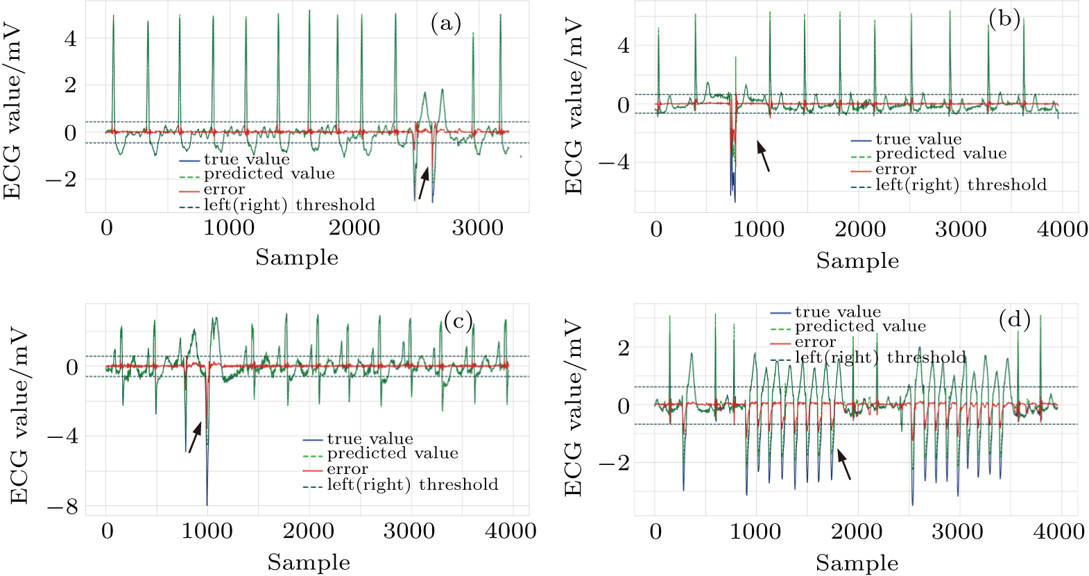 | Fig. 9. Successfully detected different kinds of anomalies in the test set, (a) ventricular couplets, (b) unclassifiable beat, (c) fusion of ventricular and normal beat, (d) ventricular tachycardia. |
The experiment is carried out with Intel Core i7-8700 K CPU @3.70 GHz, 32GB RAM, GeForce GTX 1080 Ti GPU, and our network is built based on TensorFlow. It takes an average of about 10 min to train the model, and about 1.5 min to test the 30-min data offline.
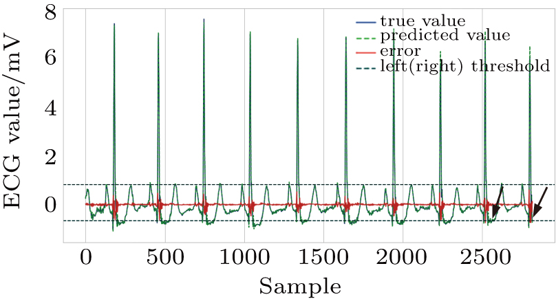
Among the methods for solving two-class classification with an ECG segment as a unit, our proposed method seems to be conservative, and the obtained ESR 53.89% in the test is not very high. This is due to our strict method constraint that FN must be extremely close to zero. Under such a strict condition, the error threshold interval is narrower and the prediction errors of the normal points are easier to exceed the threshold interval and be misjudged to abnormal, as shown in Fig.
Moreover, in terms of test set size, our method is tested on 16 complete 30-min sequences from MIT-BIH arrhythmia database, and the test results corresponding to each patient were given, while Chauhan and Vig[8] only mentioned a 20-min sequence consisting of several positive and negative ECG segments for test. Thus it is unfair to compare two methods straightly.
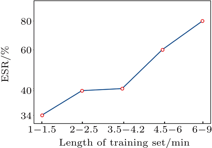
On the other hand, our test is limited by the data length of MIT-BIH database. For some test data we can find long continuous normal sequence in them, but for others such as data 105, 210, 213, we can only pick out continuous normal sequences of about 1 min. This is why we take different lengths of normal sequences in the above training and the length of the training set cannot be uniformly fixed for all patients. However, in practical wearable applications, it is believed that, continuous normal sequences usually occupy a large certain proportion in Holter data.
We do further analysis to the influence on the screening result of our problem. According to the length size of the training sequences in the experiment, samples are divided into five class, letting the number of training sequences in each class is 3–4 (each class approximately has equal samples). Then, the mean values of ESR in each class are respectively counted, as shown in Fig.
In the above experiments, such as Nos. 223 and 213, the length of the training set is below 2.5 min, so that the corresponding effective screening rate (ESR) is negatively affected. However, it is also observed that a small training set does not necessarily results in a poor experiment result, such as No. 219.
Among the existing analysis methods of ECG segments, the knowledge of abnormal data is usually needed to determine the judgment threshold, but the actual disease data is rare. Also, for clinical monitoring requirements, it should be ensured that abnormal data will not be misjudged as normal data. We have innovatively proposed a preliminary anomaly screening method for Holter data based on the LSTM model.
In our proposed method, the LSTM model is utilized to learn the pseudo-periodic mode of the normal ECG signal points, and the kernel density estimation method is utilized to calculate the probability density of prediction errors of normal data. Based only on the normal signal points, we can achieve the threshold interval that distinguishes the abnormal segments from the normal ones.
The experiments show that the proposed method can filter out a large number of normal segments that do not require further analysis, reducing the workload of subsequent multiple disease classifications. It achieves a certain effect of distinguishing normal and abnormal conditions. The stability of the model is good. The average effective screening rate obtained by repeated tests is 53.89%. The normal segments are excluded to a large extent while ensuring that no abnormal signal point is missed.
For the multi-channel ECG data, our model only needs to change the input dimension on the basis of the number of channels, and it can work.
| [1] | |
| [2] | |
| [3] | |
| [4] | |
| [5] | |
| [6] | |
| [7] | |
| [8] | |
| [9] | |
| [10] | |
| [11] | |
| [12] | |
| [13] | |
| [14] | |
| [15] | |
| [16] |


