
Nonlocal symmetries and similarity reductions for Korteweg–de Vries–negative-order Korteweg–de Vries equation
Cite this Article
Hu Heng-Chun, Liu Fei-Yan. Nonlocal symmetries and similarity reductions for Korteweg–de Vries–negative-order Korteweg–de Vries equation. Chinese Physics B, 2020, 29(4): 040201 
Permissions
Nonlocal symmetries and similarity reductions for Korteweg–de Vries–negative-order Korteweg–de Vries equation
† Corresponding author. E-mail:
Project supported by the National Natural Science Foundation of China (Grant No. 11471215).
Abstract
The nonlocal symmetries are derived for the Korteweg–de Vries–negative-order Korteweg–de Vries equation from the Painlevé truncation method. The nonlocal symmetries are localized to the classical Lie point symmetries for the enlarged system by introducing new dependent variables. The corresponding similarity reduction equations are obtained with different constant selections. Many explicit solutions for the integrable equation can be presented from the similarity reduction.
1. Introduction1 ) and (2 ) by the Hirota bilinear form and showed that it is integrable in the sense of admitting the Painlevé property. The N-th Bäcklund transformation and soliton-cnoidal wave interaction solutions for the KdV–nKdV equation has been studied in Ref. [26].
The well-known KdV equation is one of the most important integrable systems in the soliton theory and has been studied extensively since it is proposed to describe the shallow water wave propagation with small but finite amplitudes.[1] The classical Lie symmetry and nonclassical Lie symmetry methods are very effective to find the exact solutions of a given nonlinear system. But these classical symmetry methods can only involve the independent, dependent variables and their derivatives.[2] In order to find much more interaction solutions among solitons and other complicated wave solutions for the nonlinear systems, many authors proposed the nonlocal symmetry by the Bäcklund transformation, the Möbius invariant form, the Painlevé truncation expansion, and the Darboux transformation. Many new interaction solutions among different types of nonlinear excitations including the solitons, cnoidal waves, Airy waves, and Bessel waves for a number of integrable systems, such as the Kadomtsev–Petviashvili equation, the Burgers equation, the modified Kadomtsev–Petviashvili equation, and the coupled integrable dispersionless equation, are constructed by means of the nonlocal symmetry.[3–19] We should point out that these new interaction excitations have not been yet obtained by other traditional methods, such as the inverse scattering transformation, the Hirota bilinear method, and the separation variable approach.
Recently, many integrable negative-order nonlinear systems have been studied in the field of soliton theory and some relevant branches of physical phenomena.[20–22] The author proposed and constructed the exact solutions of a special integrable equation combining the well-known KdV equation and the negative-order KdV (KdV–nKdV) equation in Ref. [23]. The KdV–nKdV equation is given in the form


In this paper, we focus on the nonlocal symmetry and similarity reduction equation for the integrable KdV–nKdV equation by the Painlevé truncation method and the classical Lie symmetry method. The nonlocal symmetry for the KdV–nKdV equations (
This paper is organized as follows. In Section
2. Nonlocal symmetries and their localization for the KdV–nKdV equations (1 ) and (2 )4 ) into Eqs. (1 ) and (2 ) and vanishing all the coefficients of different powers of ϕ==(x,t) independently, we have
3 ) and (4 ) is just an auto-Bäcklund transformation between the solutions {u2, v2} and {u, v} if the function ϕ satisfies the consistent condition (8 ). Then the nonlocal symmetry of Eqs. (1 ) and (2 ) can be read out directly from the truncated Painlevé expansion of Eqs. (3 ) and (3 ) with Eq. (5 )
9 ) is
10 ), we can introduce four dependent variables by requiring
1 ), (2 ), (6 ), (7 ), and (11 ) has the form
13 ) for the enlarged system of Eqs. (1 ), (2 ), (6 ), (7 ), and (11 ) can be written as
1 ) and (2 ) with the trivial solution u2 = v2 = 0. If selecting the nontrivial seed solution and different types of the function ϕ in Eq. (8 ), one can obtain much more exact solutions of Eqs. (1 ) and (2 ).
In this section, we give the nonlocal symmetry and corresponding finite symmetry transformation for the KdV–nKdV equations (


3. Similarity reduction related to the nonlocal symmetry (9 )15 )–(22 ) are invariant under the transformation
1 ) and (2 ). In order to find the similarity variables and the corresponding reduction equation, we should solve the characteristic equation with the expressions in Eqs. (25 ). Because of the existence of six arbitrary constants in Eqs. (25 ), we consider two cases respectively.27 ) into Eqs. (6 ), (7 ), (8 ), and (11 ), we can obtain the invariant functions {U, V, Φ, G, H, P, Q} in the form
1 ) and (2 ) are obtained easily by selecting proper arbitrary constants
31 ) is given in Fig. 1 with proper constant selection and it should be pointed that this solution has singularity point when t → −1.
28 ). Substituting the expressions (33 ) into Eqs. (6 ), (7 ), (8 ), and (11 ), the invariant functions {U, Φ, V, G, H, P, Q} should satisfy the following relations
34 ) are known, the corresponding exact solutions of the KdV–nKdV equations (1 ) and (2 ) are simply obtained
26 ) with c1 = 0 are solved in the following

38 ) into Eqs. (6 ), (8 ), and (11 ), the functions 

39 ) has the simple travelling wave solution
1 ) and (2 ) can be obtained from the last two equations in Eq. (38 )
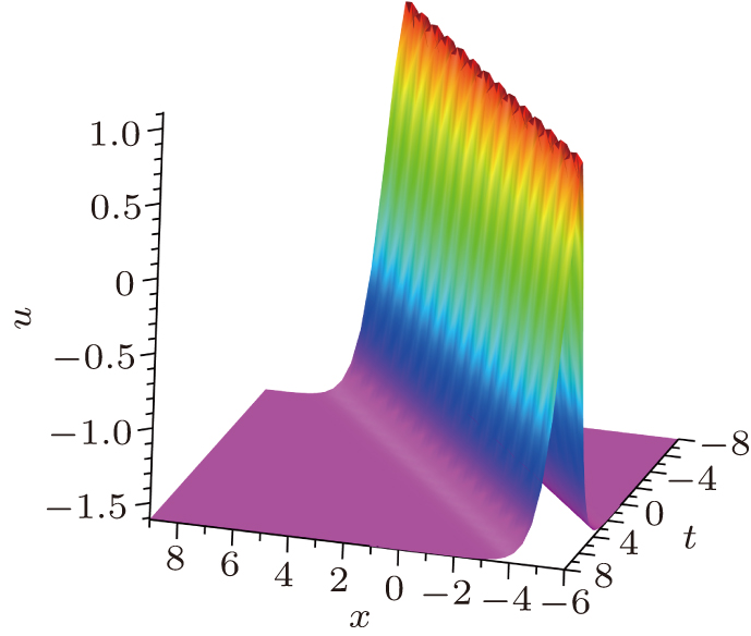
41 ) is shown in Fig. 2 with proper constant selection and the structure for v in Eq. (41 ) is similar to u which is omitted here for simplicity.

37 )
39 ) can degenerate to Eq. (45 ) when Δ = 0. But the similarity solutions for u and v are different because there exists a hyperbolic function in Eqs. (41 ) and (42 ). When we select the simple travelling wave solution as Eq. (40 ) for the similarity equations (39 ) and (45 ), the similarity solutions for u and v are the periodic solitary wave solutions and the rational function solutions respectively.
The nonlocal symmetry for the KdV–nKdV equation cannot be used to construct explicit solution directly because of the difficulty to find the nontrivial solutions of the consistent condition (


As the standard steps of the Lie symmetry method, the symmetry components σn (n = u,v,ϕ,g,h,p,q) can be supposed to have the form


Substituting the symmetry expression (


If the solution of Eq. (

A simple solution of Eq. (


 | Fig. 1. The quasi-solitary wave solution u expressed by Eq. ( |
When 


 | Fig. 2. The solitary wave solution u expressed by Eq. ( |
In the similar way, the symmetry reduction of the KdV–nKdV equations (


In the both two cases, the main parts of the reduction equations are the same except the nonlinear term with the constant Δ. It is difficult to find the exact solutions of the reduction equations because of the transcendental function solutions in equations (
4. Summary and discussion
In summary, the nonlocal symmetries for the KdV–nKdV equations (
Reference
| [1] | |
| [2] | |
| [3] | |
| [4] | |
| [5] | |
| [6] | |
| [7] | |
| [8] | |
| [9] | |
| [10] | |
| [11] | |
| [12] | |
| [13] | |
| [14] | |
| [15] | |
| [16] | |
| [17] | |
| [18] | |
| [19] | |
| [20] | |
| [21] | |
| [22] | |
| [23] | |
| [24] | |
| [25] | |
| [26] | |
| [27] | |
| [28] | |
| [29] | |
| [30] |