
Electronic structure from equivalent differential equations of Hartree–Fock equations
Cite this Article
Lin Hai. Electronic structure from equivalent differential equations of Hartree–Fock equations. Chinese Physics B, 2019, 28(8): 087101 
Permissions
Electronic structure from equivalent differential equations of Hartree–Fock equations
† Corresponding author. E-mail:
Abstract
A strict universal method of calculating the electronic structure of condensed matter from the Hartree–Fock equation is proposed. It is based on a partial differential equation (PDE) strictly equivalent to the Hartree–Fock equation, which is an integral–differential equation of fermion single-body wavefunctions. Although the maximum order of the differential operator in the Hartree–Fock equation is 2, the mathematical property of its integral kernel function can warrant the equation to be strictly equivalent to a 4th-order nonlinear partial differential equation of fermion single-body wavefunctions. This allows the electronic structure calculation to eliminate empirical and random choices of the starting trial wavefunction (which is inevitable for achieving rapid convergence with respect to iterative times, in the iterative method of studying integral–differential equations), and strictly relates the electronic structure to the space boundary conditions of the single-body wavefunction.
1. Introduction
Exactly solving the wavefunction of a quantum many-body system is the kernel task of several main branches of modern physics, such as that of nuclear structures in nuclear physics,[1,2] and that of the electronic structures of multi-electron atoms, molecules[3] and solids[4] in condensed matter physics. The difficulty in solving true/exact wavefunctions has promoted the progress of various approximation methods.[5–37] The Hartree–Fock (HF) equation is among the most widely used of these methods. Its kernel approximation is that the wavefunction of a many-fermion system can be expressed by the Slater determinant of the single-fermion wavefunction[5–7] as well as its various linear combinations.[8,9] Consequently, solving a multi-body wavefunction is simplified into solving the single-body wavefunction in a self-consistent field.
As an integral–differential equation, the HF equation is naturally attacked by the iterative method, the most popular method of solving integral–differential equations. Although this is a universal method, its efficiency is limited because achieving fast convergence of trial solutions with respect to the iterative times requires empirically and skillfully choosing the starting trial solution. If the convergence requirement is expressed as 


This difficulty promotes solution of the integral–differential equation through its corresponding partial differential equation (PDE). The merit of doing so is to avoid having to empirically and randomly choose the starting trial solution and instead relate a strict solution to the conditions for determining a solution. But such a corresponding PDE is often based on approximations. For example, in density functional theory (DFT),[10–16] the kernel approximation is to assume the integral term in the HF equation equals a summation of the products of single-body wavefunctions in finite number and hence transforms an integral–differential equation into a PDE with the same order (still a 2nd-order PDE). As shown below, if the single-body wavefunction is described with a PDE, the PDE should be at least 3rd-order, rather than 2nd-order.
Compared with the iterative method, the stricter method of solving the integral–differential equation solves its strictly equivalent PDE. For an integral–differential equation whose partial differential operatorʼs maximum order is N, it should be mathematically equivalent to at least an (N+1)-th-order PDE. Therefore, the HF equation, the maximum order of whose differential operator is 2, should be mathematically equivalent to at least a 3rd-order PDE of the single-body wavefunction. In the following section, a strict theory indicates that the HF equation is equivalent to a 4th-order PDE.
2. Theory and method
2.1. Main idea
where the two real-valued functions UL and Uc satisfy the Poisson equations (Ql and Rl are the charge and the position of the l-th ion) and the complex-valued function

reads as
where w is defined as

. Here, because the summations over q and over k + q are different expressions of the same object, w is k-independent. Besides the HF equation, each

also satisfies
where

is the volume of a cell, a is the lattice constant, VFS is the volume of the Fermi sphere, and

is the total ionic charge per cell. Moreover, the

are orthogonal to each other.
where Ek is space-independent and also time-independent. All terms in this form belong to one of two classes: one is k-dependent and the other k-independent. The condition for an equation in such a form having solutions at any k-value is that all k-independent terms in Eq. (4 ) form a closed relation and the k-dependent terms are governed by a few k-independent terms,

where E0 is the corresponding atomic level of those extended-states and **

is a constant

. Equation (5 ) is a 2nd-order linear PDE of w, and its solution is determined by a physical boundary condition

which means the density of valence electrons at the cation position is 0. Moreover, the linearity of Eq. (5 ) can warrant

to be satisfied easily by multiplying the solution of Eq. (5 ) by a constant.
where
Having obtained the expressions of VS and VC in terms of sk and

from Eqs. (7 ) and (8 ), we can substitute them into Eqs. (9 ) and (10 ) and have
Comparing the

-dependent terms, as well as the

-dependent terms, in Eqs. (14 ) and (15 ), we obtain 4 equations respectively for their

-dependent terms and

-dependent terms. The four equations are in fact 2 pairs and in each pair the two equations are the same because one is merely the other multiplied by a constant. Thus, we obtain two equations:
Note that equations (16 ) and (17 ) are a 4th-order linear PDE set of sk. Therefore, equation (3 ) can be easily satisfied by multiplying the solution of Eqs. (16 ) and (17 ) by a constant.
The single-electron wavefunction in solids is identified by wavevector k. The HF equation of 
 |
 |
 |
In DFT,[10–16] the exchange–correlation energy 


Actually, it is unnecessary to depend on those assumptions for 


 |
 |
 |
Due to the (1/r)-dependent part of the operator 


After knowing the profile of the total particle density 


 |
 |
 |
 |
 |
 |
 |
 |
 |
 |
 |
Here, we utilize the formulas
 |
 |
Equations (


2.2. Detailed mathematics
Because of Eqs. (20 ) and (21 ), there exist
and
and

and
read as
Moreover, from Eq. (17 ), we can express

as
where analytic functions C0 and C1 are defined as
Solutions of Eqs. (


 |
 |
Equations (


 |
 |
 |
 |
 |
Using the power series of 


 |
 |
 |
 |
 |
 |
 |
Thus, 
 |
or
 |
Equation (
 |
This requirement leads to
 |
2.3. Main theoretical results
Because of the formulas
we finally obtain a quadratic equation of

as follows:
where
Equations (
 |
 |
 |
 |
 |
 |
 |
Equation (
 |
2.4. Feasibility of extension to more realistic anisotropic case
where
with

being dependent on **

. Note that **

and the spherical harmonic function

satisfy a common equation
Therefore, corresponding to the expression in Eq. (45 ), w and sk have similar expressions

. Namely, when UL is

-dependent, equation (4 ) will correspond to a set of equations, each of which is for all terms associated with

. The radial coefficient function

in each
can be solved from this set, where

. Note that those

-components should warrant
Thus, for

-dependent

, we can solve, in a procedure similar to that presented previously,

and

from the

-related terms of Eqs. (5 ) and (6 ).
The same procedure can be extended to more realistic anisotropic cases. UL is 
 |
 |
 |
 |
 |
 |
3. Numerical results and discussion
Because an HF equation is a differential–integral equation, its Green function (GF) will contain infinite terms related to the unperturbed GF which is associated with a differential equation. Although many terms are small enough to be negligible, their number is so large that their summation is not negligible. Therefore, the GF of an HF equation is difficult to exactly solve. If the HF equation is approximated as a differential equation by making assumptions for 
In contrast, our method does not require any assumption for 
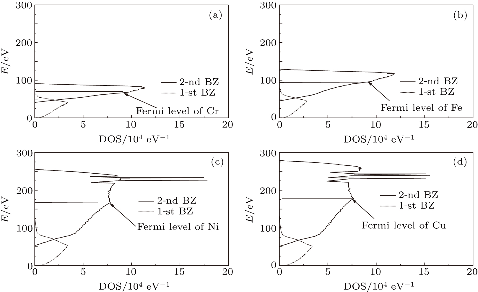
We use this method to calculate the 3d-band of a transition metal, i.e., the dimensionless parameter is chosen to be 
According to the solutions of Eqs. (


 | Fig. 1. DOS curves. |
 | Fig. 2. Values of DOS at Fermi level. |
4. Conclusions
Solving an integral–differential equation through its strictly equivalent PDE is stricter and more efficient than directly applying an iterative method to it. For the HF equation, that its Coulomb-type integral kernel function obeys the Poisson equation determines its equivalence to a 4th-order nonlinear PDE. According to the standard theory of the PDE,the solution of such a 4th-order PDE depends on its boundary conditions. Having converted the differential–integral equation into its equivalent higher-order differential counterpart according to the standard strict procedure described in the text, we can find that the equivalent differential equation contains “potentials” of space singularity 

Reference
| [1] | |
| [2] | |
| [3] | |
| [4] | |
| [5] | |
| [6] | |
| [7] | |
| [8] | |
| [9] | |
| [10] | |
| [11] | |
| [12] | |
| [13] | |
| [14] | |
| [15] | |
| [16] | |
| [17] | |
| [18] | |
| [19] | |
| [20] | |
| [21] | |
| [22] | |
| [23] | |
| [24] | |
| [25] | |
| [26] | |
| [27] | |
| [28] | |
| [29] | |
| [30] | |
| [31] | |
| [32] | |
| [33] | |
| [34] | |
| [35] | |
| [36] | |
| [37] | |
| [38] | |
| [39] |