


Phase transitions of the five-state clock model on the square lattice
Cite this Article
Chen Yong, Xie Zhi-Yuan, Yu Ji-Feng. Phase transitions of the five-state clock model on the square lattice
. Chinese Physics B, 2018, 27(8): 080503 
Permissions
Phase transitions of the five-state clock model on the square lattice
† Corresponding author. E-mail:
Project supported by the Fundamental Research Funds for the Central Universities, China (Grant No. 531107040857), the Natural Science Foundation of Hunan Province, China (Grant No. 851204035), and the National Natural Science Foundation of China (Grant No. 11774420).
Abstract
Using the tensor renormalization group method based on the higher-order singular value decomposition, we have studied the phase transitions of the five-state clock model on the square lattice. The temperature dependence of the specific heat indicates the system has two phase transitions, as verified clearly by the correlation function at three representative temperatures. By calculating the magnetic susceptibility, we obtained only the upper critical temperature as Tc2 = 0.9565(7). Investigating the fixed-point tensor, we precisely locate the transition temperatures at Tc1 = 0.9029(1) and Tc2 = 0.9520(1), consistent well with the Monte Carlo and the density matrix renormalization group results.
1. Introduction
The research on exotic phases and the phase transitions has always been one of the central topics in statistical and condensed matter physics.[1] A typical example is the continuous XY model on the square lattice, which has attracted much attention since Kosterlitz and Thouless (KT),[2,3] discovered a phase transition at finite temperature without any symmetry breaking, obviously beyond Landau’s symmetry breaking theory for continuous phase transitions. Its low temperature phase, characterized by the bound vortex–antivortex pairs, is called the quasi-ordered or topological phase, with a divergent correlation length. The transition to the high temperature disordered (or paramagnetic) phase is attributed to the unbinding of these topological pairs.[2,3]
Its discrete version, the q-state clock model exhibits even richer features in phase transitions, dependent on q, and arouses extensive interests and debates consequently. As is well known, if q ⩽ 4, the model has only one order-disorder transition of Ising type; when q approaches infinity, it then transits to the continuous XY model, with one KT transition.[4] Furthermore, it is agreed that there exists a critical qc, once q ⩾ qc, the system has two transitions, separated by the topological KT phase in-between. Apparently, the discrete symmetry plays an important role on the transitions. There has been a large amount of studies on this model with different q’s.[5–18]
So far, still there are debates on the very value of qc, though many believed to be 5. Besides, the precise determination of the transition temperatures and types is also inconclusive. An early renormalization group (RG) analysis suggested two KT-type transitions[19] for q = 5 case. Another recent density matrix renormalization group (DMRG) calculation[20] with maximum size L = 256, estimated these two KT transition temperatures as Tc1 = 0.914(12) and Tc2 = 0.945(17) respectively. While, Monte Carlo (MC) simulations even gave inconsistent conclusions among themselves,[10,13,15,21,22] mainly due to a different usage of the boundary twist and the physical quantities investigated to characterize the transitions, details in Refs. [21], [22], and [13]. For the transition temperatures, Borisenko et al.[15] obtained Tc1 = 0.90514(9) and Tc2 = 0.95147(9) with size up to L = 1024, by calculating the susceptibility; and Kumano et al.[21] predicted Tc1 = 0.908 and Tc2 = 0.944 using largest size L = 256, with investigation of the helicity modulus. All methods deal with relatively small system sizes.
In recent years, the tensor network states method has developed rapidly and become one of the most powerful numerical tools to study the phase transitions in both the classical and the quantum many-body systems.[23–29] The tensor renormalization group method based on the higher-order singular value decomposition (abbreviated as HOTRG),[28] has been applied successfully to the continuous XY model,[30] the 3-dimensional Ising model[28] and the Potts model.[31,32]
In this article, we have investigated the phase transitions of the ferromagnetic five-state clock model on the square lattice by the HOTRG method. Firstly, by inspecting the specific heat and the spin–spin correlation, we confirmed that this model indeed has two phase transitions, separated by a narrow interval characterized with a power law correlation, apparently different to the low- or high-temperature Ising-type phases. Then we investigated the magnetic susceptibility, with performing a bond dimension scaling, only the upper transition temperature is obtained, at Tc2 = 0.9565(7). Finally, by studying the property of the fixed-point tensor from the RG flow, these two transition temperatures are located precisely at Tc1 = 0.9029(1) and Tc2 = 0.9520(1) respectively. The results agree quite well with the MC[15,21] and the DMRG[20] predictions.
The article is organized as follows: Section
2. Model and method
The Hamiltonian of the ferromagnetic q-state clock model with an external magnetic field is defined as
For a classical statistical system, the tensor network states method usually starts by expressing the partition function as a product of all local tensors
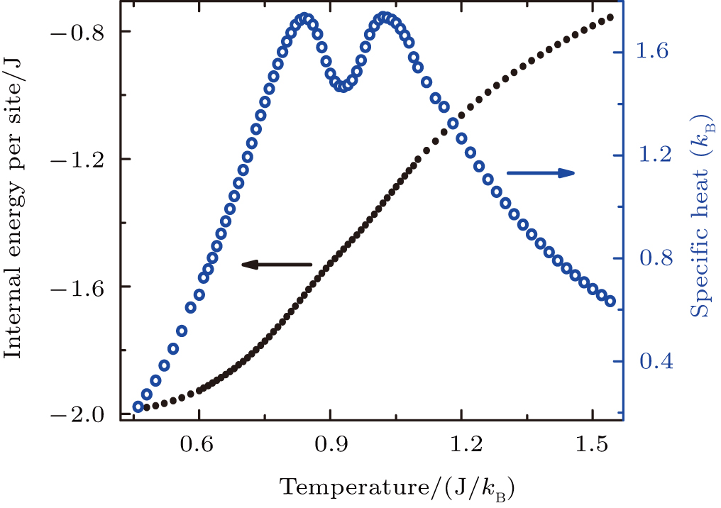
 | Fig. 1. (color online) Temperature dependence of the internal energy and the specific heat with h = 0 and D = 40. Two obvious peaks indicate two possible phase transition from the specific heat. |
We should again note that the HOTRG is credited for handling big size systems. Only log2N steps are needed for the full contraction, given size N, which then could be very large to approximate the thermodynamic limit, and thus avoid the error inherent in the finite size scaling. In this work, we run the coarse-graining process until each physical quantity has converged. Normally, it takes 40 to 60 steps, so the system size is 240 to 260, approaching the infinity. One more thing should be mentioned is the size of the local tensor’s legs, or the bond dimension denoted as D, is equal to q initially. During each RG step, it is expanded quickly, then truncated to guarantee the process manageable. Usually, bigger the bond dimension, better the accuracy.
3. Results and discussions
As illustrated in Fig.
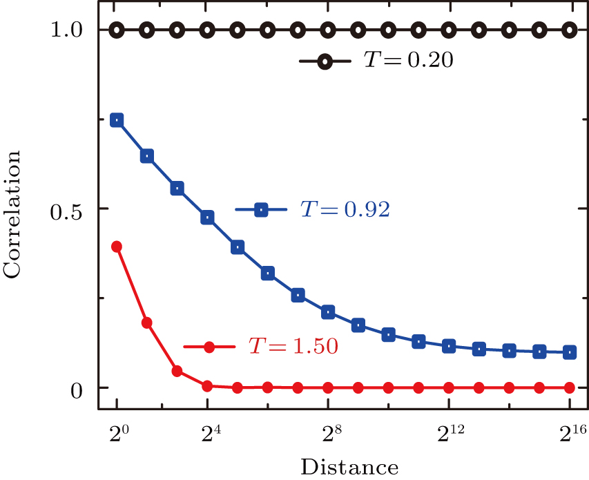 | Fig. 2. (color online) Spin–spin correlation along the horizontal direction with D = 40. Three different behaviors, each characterizing one phase respectively, can be distinguished clearly. |
The specific heat cannot be used to determine the transition points, for which is derivatively continuous, as in the classical XY model on the square lattice, and thus whose peaks do not correspond to the transition temperatures. We then turn to investigate the system’s response to a static weak external magnetic field. We first evaluate the magnetization per spin, as shown in Fig.
 | Fig. 3. (color online) Magnetization with existence of weak external magnetic fields, and the corresponding magnetic susceptibility as defined in Eq. ( |
From the magnetization, we can calculate the magnetic susceptibility
Following the procedure in Ref. [30], for a given D, we can determine the transition temperature by locating the peak positions of the magnetic susceptibility with respect to the external fields, and then extrapolating to the zero-field limit. As only one peak shows up, the upper transition between the quasi-ordered and the disordered phases is then predicted at Tc2 = 0.9561(10) by a power law fitting for D = 40, as presented in Fig.
 | Fig. 4. (color online) The peak position of the magnetic susceptibility with respect to the external field, and a power law fitting is also performed for extrapolation to zero-field limit. The critical point is obtained as Tc2 = 0.9561(10) for D = 40 case. |
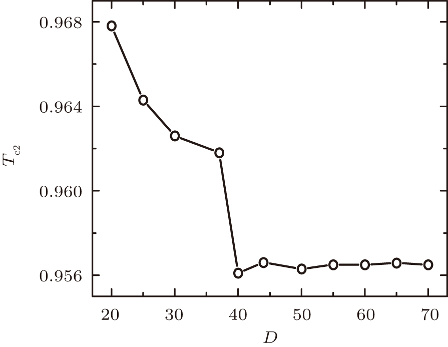 | Fig. 5. (color online) The upper phase transition temperature with respect to the bond dimension D by the magnetic susceptibility calculation. The converged transition temperature is Tc2 = 0.9565(7). |
For a complete description of the transition temperatures, we turn to focus on the local fixed-point tensor. At each coarse-graining step, an optimized isometric matrix is obtained to truncate the expanded tensors. Eventually, each local tensor flows to a corresponding fixed-point tensor. One can fetch information from the fixed-point tensors, as first introduced in Ref. [25] to identify the different phases of the Ising model, where a gauge invariant quantity X is defined as
Taking D = 75 for an example, the calculated X is shown in Fig.
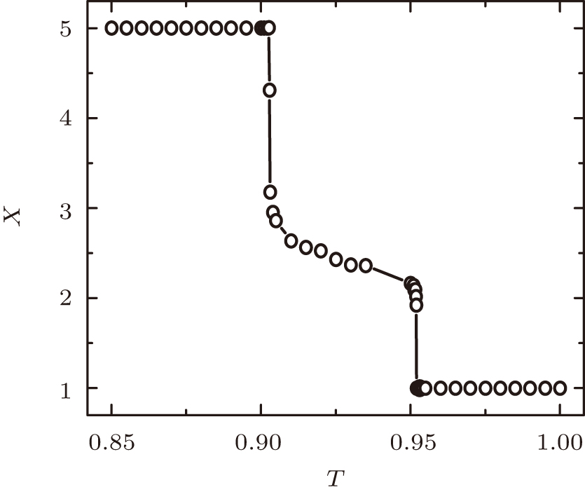 | Fig. 6. (color online) Temperature dependence of X obtained from the fixed-point tensors, which shows two jumps around T1 = 0.903 and T2 = 0.952. The results are obtained with D = 75 as an illustration. |
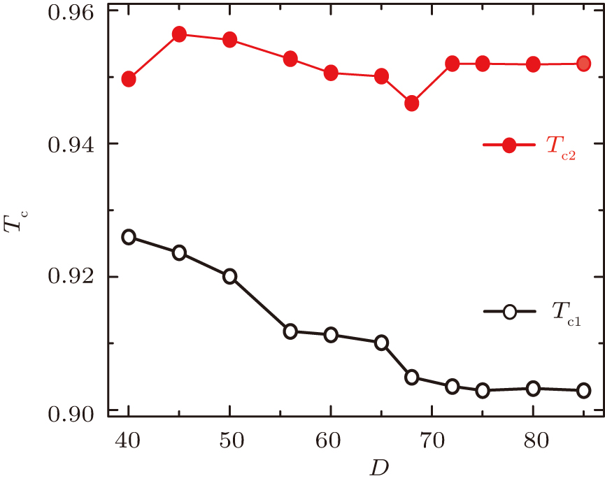 | Fig. 7. (color online) The lower and upper transition temperatures with respect to bond dimensions D from X calculation. And the converged results are Tc1 = 0.9029(1), and Tc2 = 0.9520(1). |
| Table 1.
Comparison of the critical temperatures, Tc1 and Tc2 by different methods for the five-state clock model. . |
4. Conclusion
Briefly, we have studied the phase transitions of the ferromagnetic five-state clock model on the square lattice, using the HOTRG algorithm to investigate the thermodynamic observables with the existence of a weak external magnetic field, and the properties of the fixed-point tensor.
First, by calculating the specific heat and the correlation function, we confirm that there are indeed two phase transitions separating three phases: the low-temperature ordered phase, the high-temperature disordered phase, and the quasi-ordered phase in-between. Second, for a given bond dimension D, the upper transition temperature alone is determined by investigating the magnetic susceptibility. Through a scaling with different D’s, we obtained the converged transition temperature at Tc2 = 0.9565(7). In order to precisely determine both transition temperatures, we extracted X from the fixed-point tensors, which shows two clear abrupt jumps, corresponding to two phase transitions. Also with a bond dimension scaling, the converged transition points are located at Tc1 = 0.9029(1) and Tc2 = 0.9520(1) respectively, consistent with the MC[15,21] and the DMRG[20] results.
Reference
| [1] | |
| [2] | |
| [3] | |
| [4] | |
| [5] | |
| [6] | |
| [7] | |
| [8] | |
| [9] | |
| [10] | |
| [11] | |
| [12] | |
| [13] | |
| [14] | |
| [15] | |
| [16] | |
| [17] | |
| [18] | |
| [19] | |
| [20] | |
| [21] | |
| [22] | |
| [23] | |
| [24] | |
| [25] | |
| [26] | |
| [27] | |
| [28] | |
| [29] | |
| [30] | |
| [31] | |
| [32] |