† Corresponding author. E-mail:
Stochastic resonance (SR) has been proved to be an effective approach to extract weak signals overwhelmed in noise. However, the detection effect of current SR models is still unsatisfactory. Here, a coupled tri-stable stochastic resonance (CTSSR) model is proposed to further increase the output signal-to-noise ratio (SNR) and improve the detection effect of SR. The effects of parameters a, b, c, and r in the proposed resonance system on the SNR are studied, by which we determine a set of parameters that is relatively optimal to implement a comparison with other classical SR models. Numerical experiment results indicate that this proposed model performs better in weak signal detection applications than the classical ones with merits of higher output SNR and better anti-noise capability.
Owing to an increasing demand for detecting weak signals in many fields, weak character signal detection technology has gradually become a hot research topic. While traditional methods were limited to expensive devices and relatively low signal-to-noise ratio (SNR), researchers have devoted themselves to seeking another way of measuring weak character signals in strong noise. Since firstly discovered by Benzi et al. in 1981 as an explanation for the observed periodicity in the ice ages on earth,[1] stochastic resonance (SR) has attracted much attention due to its most distinct merit of enhancing the weak signal by exploiting the noise energy. During the past few decades, SR has been explored experimentally in a large variety of fields, such as physics, biology, optical systems, and large mechanical fault diagnosis.[2–6]
The cooperative effect of noise, the periodic driving in a bi-stable system, and the application of the SR system for detecting a weak signal accompanied with heavy background noise were investigated by Jung in 1991.[7] Signal amplification in a nano-mechanical Duffing resonator via SR was proposed by Gammaitoni in 1995.[8] Lutz applied SR in nonlinear signal detection in 2001.[9] Gandhimathi and Mankin studied the condition for noise energy induced signal energy to enhance weak signal detection performance.[10,11] Saikia presented a modified adaptive SR model to detect faint signals with strong noise in sensors.[12] Some other researchers discussed the issues on coupling in SR models.[13–19] Besides, SR systems with many new potential functions, like the tri-stable potential, were also explored by researchers.[20–22]
However, for these existing SR models, the output SNR is not high enough and the detection effect is still not satisfactory. The detection effect of SR refers to the noise utilization or the enhancement extent on the periodic input signals, whose evaluation index is mainly the SNR or SNRgain of the system response tracking periodic input signal in this study. In other words, the greater the noise utilization or the enhancement extent on the periodic input signals, the greater SNR or SNRgain of the system response is, and vice versa. Thus, it is necessary to search new resonance models to further improve the capability of utilizing the noise to enhance the input signal through the application of SR. Based on the studies of predecessors and by combining the coupling and tri-stable potential function, a novel coupled tri-stable stochastic resonance (CTSSR) model is proposed in this paper to improve the output SNR and detecting performance of SR systems.
This paper is organized as follows. In the next section, the principle of tri-stable stochastic resonance (TSR) is described. Then we propose our novel model and analyze the effects of the system parameters on the output SNR. In Section
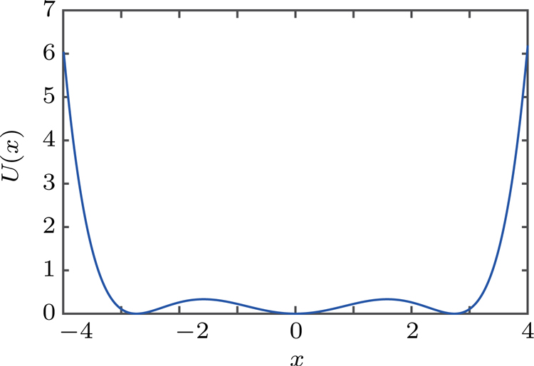
The basis of the tri-stable SR phenomenon can be described as follows. A particle is driven by a weak periodic signal and the Gaussian white noise in a tri-stable potential containing three potential wells and two potential barriers. The periodic oscillation can be enhanced when the noise is at a suitable level, which can be explained by the equation[22]
 |


For the TSR model, U(x) represents a potential function
 |
Although the output SNR is improved by using the method of tri-stable resonance, it is still not satisfactory. When the intensity of noise becomes high, the detecting performance will be poor. In order to obtain higher SNR and excellent performance, based on the traditional TSR model, we propose a novel model, CTSSR, which can be illustrated as follows:
 |
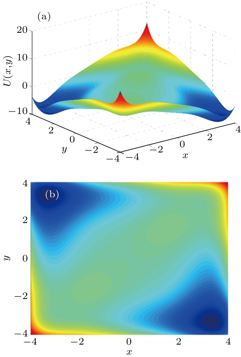
Under this circumstance, the potential function evolves into a new form
 |
Comparing Eq. (
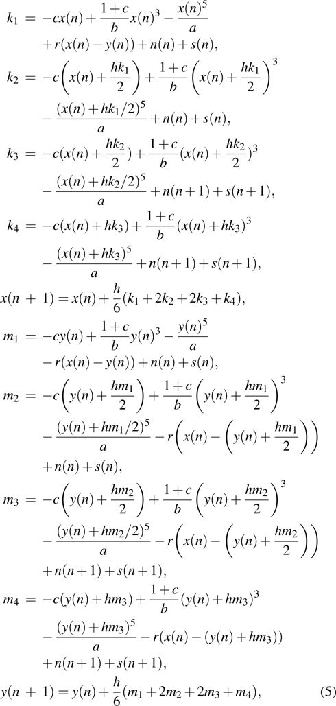
In order to meet the demand for application in practical engineering, we need to convert the continuous system into a discrete form for convenience and high efficiency. We utilize the fourth-order Runge–Kutta (RK4) algorithm to implement the discretization of the continuous system. By selecting a calculation step h, according to Eq. (
 |
 |

 |
In this study, the intensity of the input useful signal is constant, so when the noise intensity increases, SNRin will decrease, and SNRout and SNRgain will vary accordingly. Then an optimal noise intensity in this system corresponds to an optimal SNRin, leading to the highest SNRgain which obviously signifies the occurrence of stochastic resonance. Herein, with a view to the definition of SNRgain and analyzing the SR models from the point of view of SNR thoroughly, we focus on the changes of SNRgain with SNRin to evaluate the performance of the SR models. Besides, the four parameters in the CTSSR system would have an impact on the system’s performance and are variable at the same time. It is extremely hard to seek out a set of optimal parameters. Thus, we adopt the single variable method to investigate the influence of each parameter on the system SNRgain, by which we select a set of parameters that are relatively optimal to conduct the weak signal detection. In our numerical simulation, the amplitude of sinusoidal signal A is 0.3 A, the driving frequency f is 0.01 Hz, the initial phase is 0°, sampling frequency 
Firstly, we explore the effects of the parameter b. SNRgain as a function of SNR of the input signal with noise with different system parameter b and a = 25, c = 0.5, r = 0.5 is shown in Fig. 
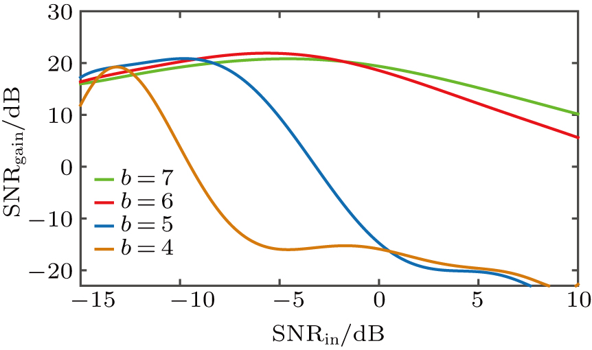 | Fig. 3. (color online) SNRgain as a function of SNRin of input noise signal with different system parameter b and a = 25, c = 0.5, r = 0.5. |
Then, the simulation experiment aiming to study the parameter a is performed, as shown in Fig.
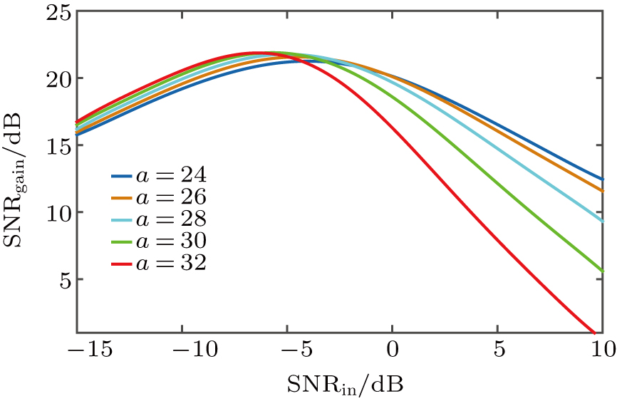 | Fig. 4. (color online) SNRgain as a function of SNRin with different system parameter a and b = 6, c = 0.5, r = 0.5. |
Figure
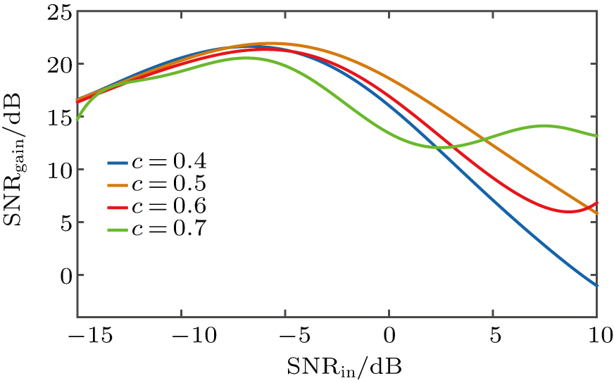 | Fig. 5. (color online) SNRgain as a function of SNRin with different system parameter c and a = 30, b = 6, r = 0.5. |
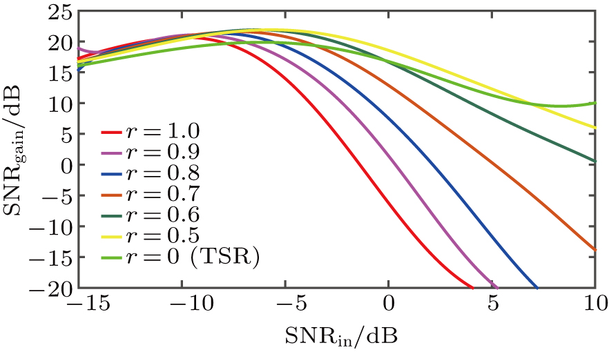
At last, we focus on the effects of r on system SNRgain, which is shown in Fig.
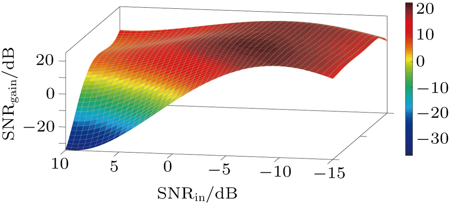 | Fig. 6. (color online) SNRgain as a function of SNRin with different system parameter r with a = 30, b = 6, c = 0.5 of CTSSR. |
From Fig.
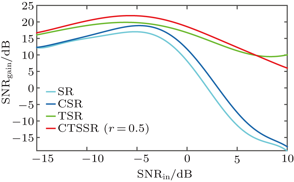
In order to prove the superiority of the CTSSR, we adopt the above parameters to conduct simulation experiments to compare it with other existing SR models, including bistable SR (SR) (a = 1 and b = 1, it is widely considered as a set of empirical values in the field of stochastic resonance which can induce excellent performance of the system), coupled bistable SR (CSR) (with four variable parameters a, b, r, and SNRin, it is difficult to seek out optimal values of the parameters in the system, and there are no studies which have ever discussed this. Accordingly, we intend to seek out an optimal value of r on the basis of keeping a = 1 and b = 1 and then make the comparison. Finally, r is determined as 0.25 in consideration of maximum SNRgain and range within which the system has excellent performance (
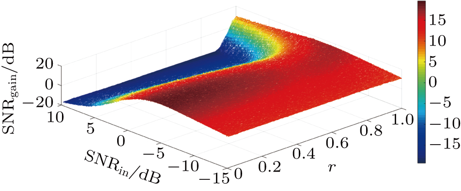 | Fig. 8. (color online) SNRgain as a function of SNRin with different system parameter r with a = 1, b = 1 of CSR. |
The superiority of CTSSR (r = 0.5) in contrast to other SR models is obvious and significant. Among almost all the range of SNRin, the SNRgain of CTSSR is the highest, indicating that the CTSSR has not only an excellent performance in improving the SNR in weak signal detection, especially under the strong noise environment, but also a better performance in detecting range. In other words, the SNR of the CTSSR system could maintain high in a wider range. Besides, we can observe that the ranking by performance in SNR from high to low is: CTSSR, TSR, CSR, and SR.
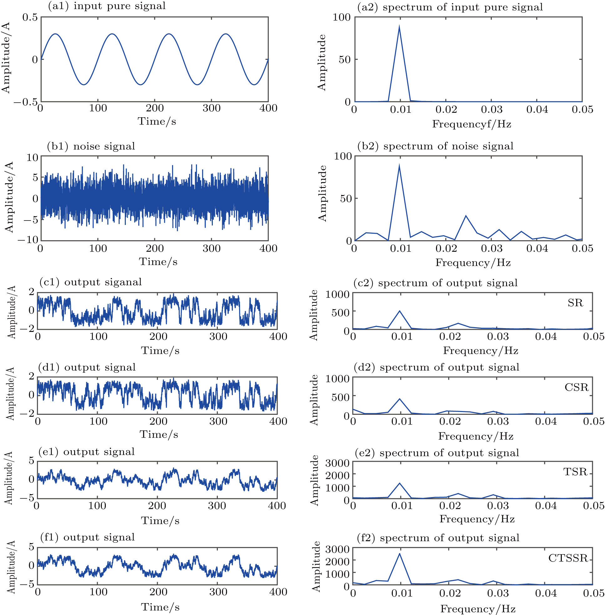
In the aspect of SNR, we are informed that the CTSSR is much better than the others. Furthermore, we implement a study in time domain and frequency domain to compare their performance. Based on the above conclusion that the CTSSR has better performance not only under relatively weak noise, but also under strong noise, to confirm this superiority, we choose different values of noise intensity D to conduct simulation experiments in both time domain and frequency domain. Firstly, we set noise intensity D = 3.0. Figures
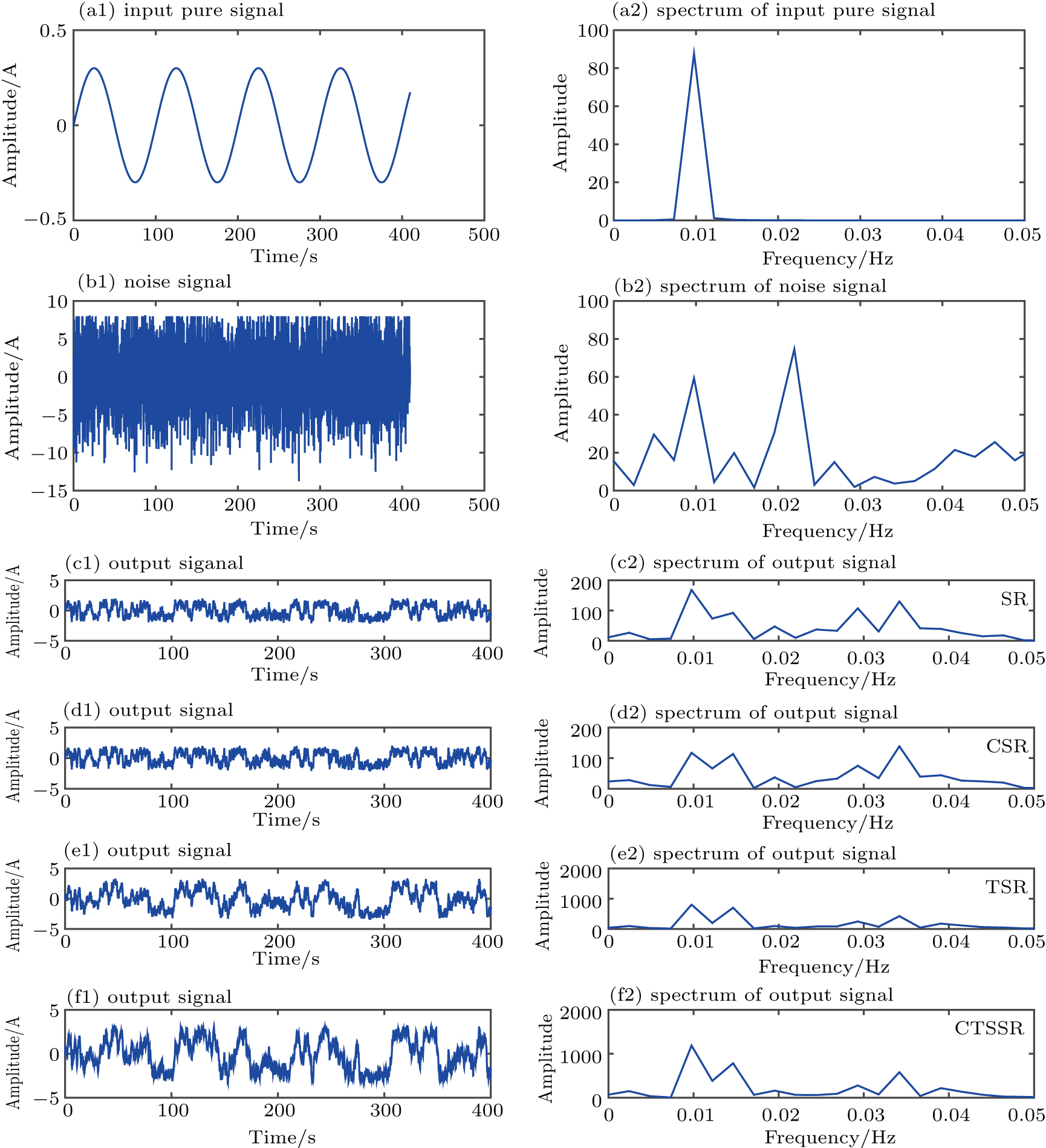
By increasing the noise intensity D to 6.0, we obtain a new telltale figure, as shown in Fig.
In this paper, a novel SR model CTSSR is proposed. We study the effects of the system parameters on its characteristics firstly and then select a set of system parameters that are relatively optimal according to its performance in SNR. Finally, the comparisons between the CTSSR and other SR models in SNR and time-frequency domain are carried out. The results of numerical experiments on SNRgain show that the SNRgain of CTSSR is higher than that of other SR models including SR, CSR, and TSR under strong background noise. It is confirmed by numerical experiments in the time and frequency domain that the ability of our proposed system in detecting a weak signal is better than that of the others, especially when the noise intensity is high. In view of all its merits, it has been proved theoretically that the proposed model is beneficial to detect a weak signal overwhelmed in strong noise. We hope it has a broad prospect of application to engineering in the future.


