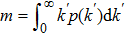
1. IntroductionMany social, communication, and information systems can be represented in terms of networks[1] — sets of nodes (or vertices) joined together in pairs by links (or edges) — with wide practical applications ranging from searching on the Internet[2] to controlling infectious diseases.[3] Research in networks has focused on the analysis of topological properties of complex systems in the real world and generating abstract models to understand microscopic mechanisms of network evolution as well as the effects of the network structure on dynamical processes.[4] Until recently, most studies in this field have been concerned with the study of static networks, ignoring the dynamic nature of realistic systems. The use of the static network is convenient for the sake of mathematical analysis, but sometimes it brings about biases in the dynamics of/on networks. Recently, much attention has been paid to temporal characteristics of networked systems[5,6] where edges vary with time.
The characterization and modelling of time-varying networks were put into practice because of availability of large data of real-time tracking of human interactions and social relationships. In this context, considering interactions in dynamic networks as a time series of events, a number of recent works focused on the statistics of events and inter-events,[7–13] and investigated their influences on diffusion and spreading processes.[14–21] On the one hand, it has been shown that the distribution of inter-event times of some communication systems follows non-Poissonian, heavy-tailed distributions, which results in bursty patterns of concurrency and duration of interactions. On the other hand, interactions in some dynamic systems are distributed homogeneously in time, e.g., switching behavior between inactive and active states in social systems. In this scenario, an important characteristic of time-varying networks is the statistics of events.
A typical model from this perspective is the activity-driven network recently proposed by Perra et al.[22] The basic premise of this model is that the formation of links is driven by the activity of nodes. They empirically obtained the distribution of individual agents’ activity in three real-world networks: Collaborations in the journal “Physical Review Letters”, messages exchanged over Twitter, and the activity of actors in movies and TV series, which allows the definition of the network dynamics based on nodes’ activity. For each node i, a fixed potential xi, the random number drawn from a given probability distribution function f(x), is assigned to measure its activity or fitness. At each time step, the network starts with N isolated nodes. Then node i becomes active with the probability proportional to xi and generates m links connecting to other random nodes. Inactive nodes can still receive connections from active ones. Since the model is random and Markovian in the sense that agents do not have memory of the previous time steps, the degree distribution of the time-aggregated networks follows the same functional form as that of the distribution f(x).[22,23] To exceed this limit, modifications of the activity-driven model have been proposed considering different scenarios, such as mutual selection,[24] memory effects,[25] strong and weak ties.[26] Although the activity-driven model is a simple representation of time-varying networks, it allows the theoretical analysis of concurrent networks and dynamical processes of interest.[27–32]
In this paper we propose an alternative activity-driven model to explain the change of individual activity and its influence on network dynamics. The model contains twofold dynamics during the evolution. First, the network grows with the addition of new nodes, which is consistent with the open feature of most real-world networks.[33] Second, all the nodes can be in one of the two states: active and inactive. Nodes transit between active and inactive states based on the collective memory.[34] Instead of considering connectivity emerging and disappearing at a given time (e.g., the birth–death process,[35]) the present model preserves previous links, but only a small fraction of them are active when the endpoints are active. To understand its reality, we take citation networks as an example. During the growth of the citation network, there are two universal features. One is the half-life effect,[36] that is, aging papers are rarely cited since they are no longer sufficiently topical. The other is the delayed recognition phenomenon,[37] which reflects papers did not seem to achieve any sort of recognition until some years after their original publication. Based on the collective memory, the published papers can be divided into two states: active and inactive. One can notice state transitions during evolution: deactivating papers based on the aging effect and activating papers based on the recognition process, and only active papers can receive citations from new papers.
2. ModelThe network contains the addition of newcomers and state transitions of nodes. Each node might receive links while it is active. Suppose that there is an initial network of n0 isolated seeds, in which m(< n0) nodes are active. The number of incoming edges of a node is denoted by the in-degree k′. At each time step, the dynamics runs as follows.
(i) Adding a new active node n with m outgoing edges that are attached to previously existing m active ones. The in-degree of the newcomer is  at first. Each selected active node l receives exactly one incoming edge, thereby
  .
.
(ii) Activating one of the previously existing inactive nodes. The probability of an inactive node i being activated is  . Meanwhile, deactivating two of the active nodes. Thus, the number of active nodes is time-unchanged. The probability of an active node j being deactivated is
  . Both μ(k′) and ν(k′) are functions of the node’s in-degree, which reflects the collective memory.
Different from the activity-driven model that previous links are not kept in the next step,[22] the present model maintains all the links and the temporal feature is defined by the activity of nodes. At each time step, only a small number m of nodes are active and a small fraction of links from the m nodes are active. Thus, instantaneous dynamical interactions take place through these active links. As the first step of research, we address the study of the aggregated network based on aforesaid two mechanisms, by using a differential equation approach. We study the degree distribution of nodes of the aggregated network. The analytical expressions are tested by numerical simulations.
3. Degree distributionDenoting with A(k′,t) and D(k′,t) the number of active and inactive nodes at time t, respectively, one can write out the differential equations for network evolution:
where
C(
k′,
t) represents the number of inactive nodes with in-degree
k′ and time
t being activated. On the right-hand side of the first equation, the first term accounts for two processes: one is the active node with in-degree
k′ at time
t attached by the newcomer in the next step, and the other is the inactive node with in-degree
k′ being activated at time
t and attached by the newcomer in the next step. The second term represents the active node with in-degree
k′ + 1 at time
t attached by the newcomer at time
t + 1. On the right-hand side of the second equation, the first term considers two processes: one is the non-selected active node with in-degree
k′ at time
t by the newcomer that is deactivated at time
t + 1, and the other is the inactive node being activated at time
t that is deactivated at time
t + 1. The second term represents the activation of inactive node with in-degree
k′ in the next step.
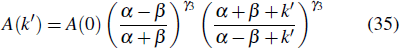
Imposing the stationary condition ∂A(k′,t)/∂t = 0 yields
For large
t, the total number of nodes in the network is approximately equal to the number of inactive nodes, and the overall in-degree distribution
p(
k′,
t) can be approximated by considering the inactive nodes only. Assuming that the limit
p(
k′) = lim
t→∞p(
k′,
t) exists, one obtains
D(
k′,
t) =
tp(
k′), and
p(
k′) can be calculated as the rate of the change of active nodes
A(
k′):
In the following, we consider both uniform and preferential activation and deactivation rates, which leads to four combinations.
3.1. Uniform activation and deactivationIn this simplest case, the activation probability of an inactive node j is
We can get the activation number of inactive nodes with in-degree
k′ at time
t as
Using the condition
D(
k′,
t) =
tp(
k′), and substituting Eq. (
6) into Eq. (
4) gives
The probability of an active node
j being selected for deactivation is
Substituting Eqs. (
7) and (
8) into Eq. (
3) yields
Therefore, we have
and obtain the solution
where
k′ ≥ 1 and the boundary value
A(0) = 1 reflects constant addition of newcomers with initial
k′ = 0. Thus, the overall in-degree distribution
p(
k′) is
To obtain the total degree distribution, we rewrite the above equation as
with
k =
k′ +
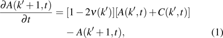
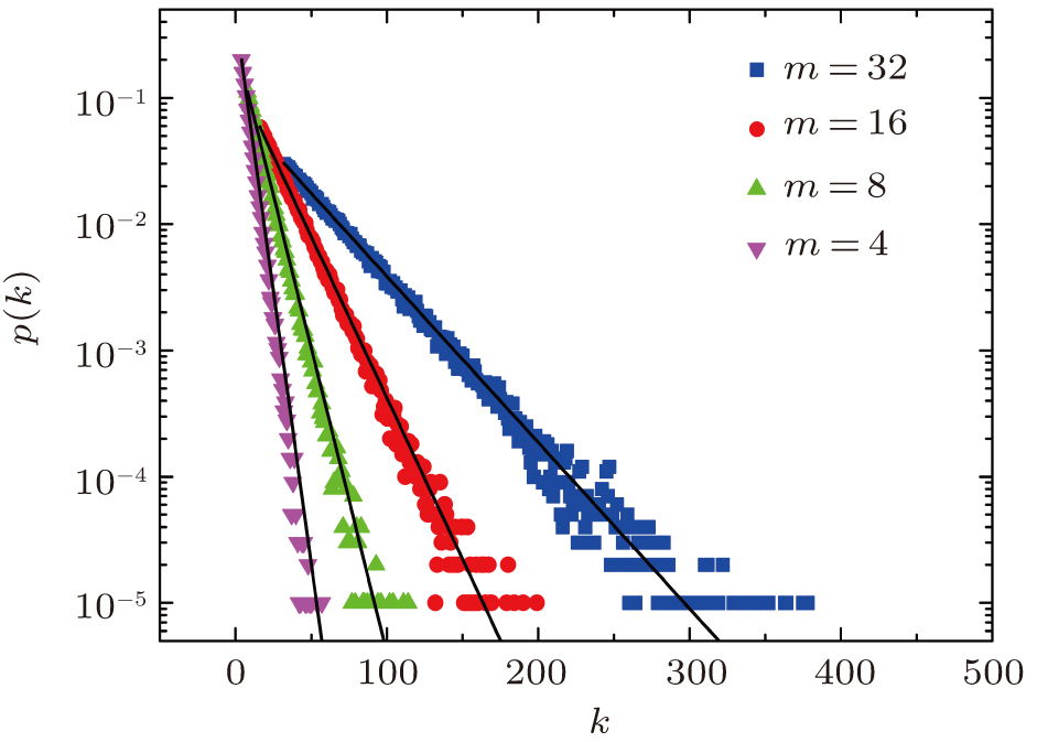
m. Thus, the distribution decays exponentially. Figure
1 shows the total degree distribution obtained by simulating the model for 10
5 time steps. As expected, one obtains exponential distributions with the exponent 1/(
m + 1), which equals 0.2, 0.11(1), 0.05(9), and 0.03(0) corresponding to
m = 4, 8, 16, and 32, respectively.
3.2. Uniform activation and preferential deactivationIn the case of preferential deactivation, the probability of an active node j being selected for deactivation is given by
where
a1 > 0 is a constant bias, and the normalization is defined as

. The summation runs over the set
Λ of the currently active nodes. Substituting Eqs. (
7) and (
14) into Eq. (
3) gives
the solution of which reads
Thus, the overall in-degree distribution
p(
k′) is
where
c1 = (
γ1 − 1)(
a1 −
γ1 + 1)
γ1−1 is the normalized factor. By rewriting the above equation, we obtain the total degree distribution
The exponent
γ1 can be obtained from a self-consistency condition
, which gives
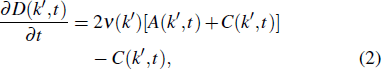
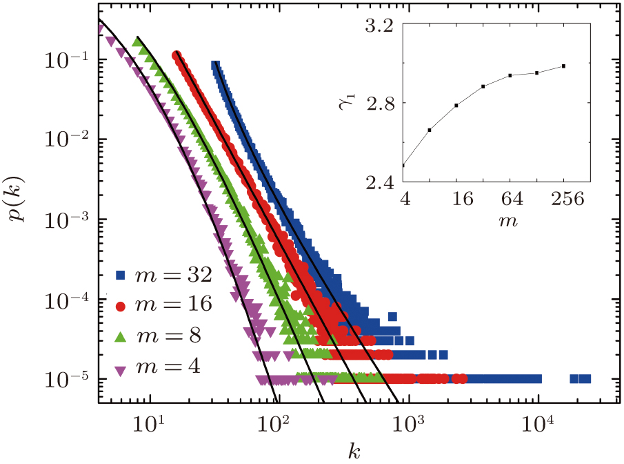
Figure 2 shows the total degree distribution obtained by simulating the model for 105 time steps in the case of a1 = 18. As expected, one obtains power-law distributions with the analytical exponent γ1 equal to 5.4, 3.88(9), 3, and 2.51(5) corresponding to m = 4, 8, 16, and 32, respectively. The inset shows the increasing behavior of γ1 as a function of m in the case of a1 = m + 2. For smaller values of m, finite size effects set in and the degree distribution shows deviations from the predicted behavior. As m increases, the discrepancy between analytical and numerical results decreases.[34] In the limiting case of large m, the continuous approach predicts the exponent 3.
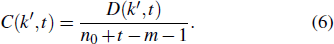
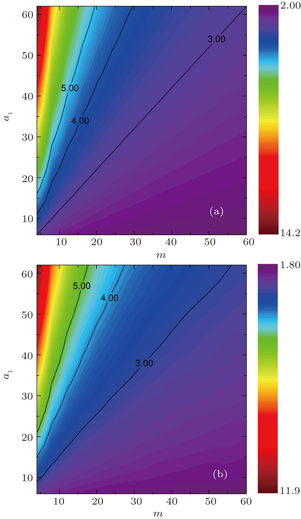
In Fig. 3, we show the influences of m and a1 on γ1 both analytically and numerically. From the shape of the contour, it can be seen that solely increasing m (a1) leads to smaller (larger) γ1. Only in the special case can γ1 equal 3. Again, numerical results are a little smaller than theoretical predictions due to the finite size effect.
3.3. Preferential activation and uniform deactivationIn the case of preferential activation, the probability of an inactive node j being selected for activation is given by
where
a2 is a constant bias and the summation runs over the set
Ω of all the currently inactive nodes. We can get that the activation number of inactive nodes with in-degree
k′ at time
t is
Using the condition
D(
k′,
t) =
t p(
k′), and substituting Eq. (
21) into Eq. (
4) yields
Substituting Eqs. (
8) and (
22) into Eq. (
3) gives
the solution of which reads
with
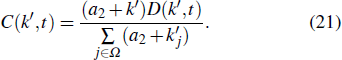
Then the overall in-degree distribution
p(
k′) is
where
c2 = (
γ2 − 1)(
a2 +
b1)
γ2 − 1 is the normalized factor. To obtain the total degree distribution, we rewrite the above equation as
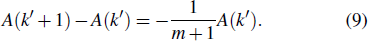
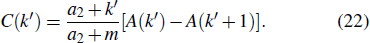
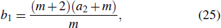
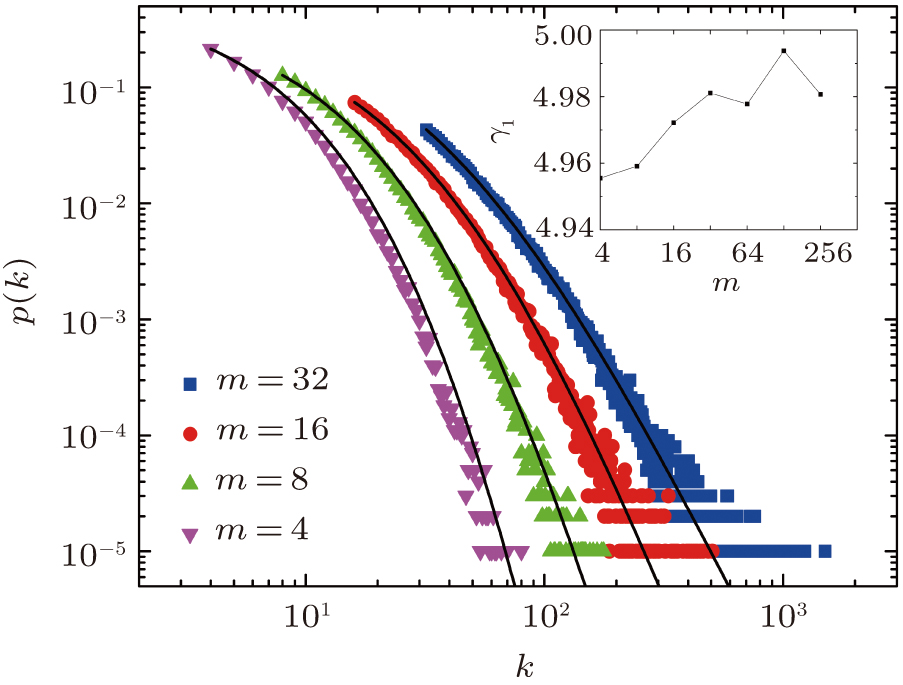
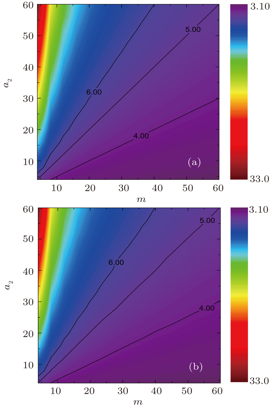
Figure 4 shows the total degree distribution obtained by simulating the model for 105 time steps in the case of a2 = 20. As expected, one obtains power-law distributions with the analytical exponent γ2, which equals 13, 8, 5.5, and 4.25 corresponding to m = 4, 8, 16, and 32, respectively. The inset shows the increasing behavior of γ2 as a function of m in the case of a2 = m. In Fig. 5, we plot γ2 in the m-a2 plane, which shows the influence of the competition of two ingredients on the exponent.
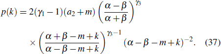
3.4. Preferential activation and deactivationFor the preferential activation and deactivation rates, one substitutes Eqs. (14) and (22) into Eq. (3), and obtains
with
Then, one has
with
The solution of Eq. (32) is
with
γ3 = (
γ1 − 1)(
a2 +
m)/
β. Thus, the overall in-degree distribution
p(
k′) is
Meanwhile, the total degree distribution can be written as
Since it is difficult to solve
γ1 from the self-consistency condition, we compute it by numerical simulations.
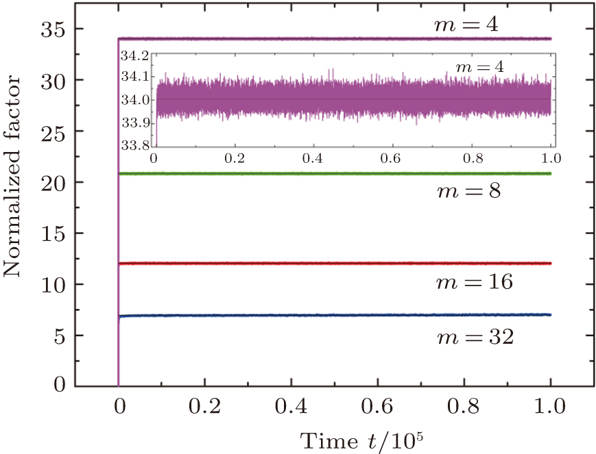
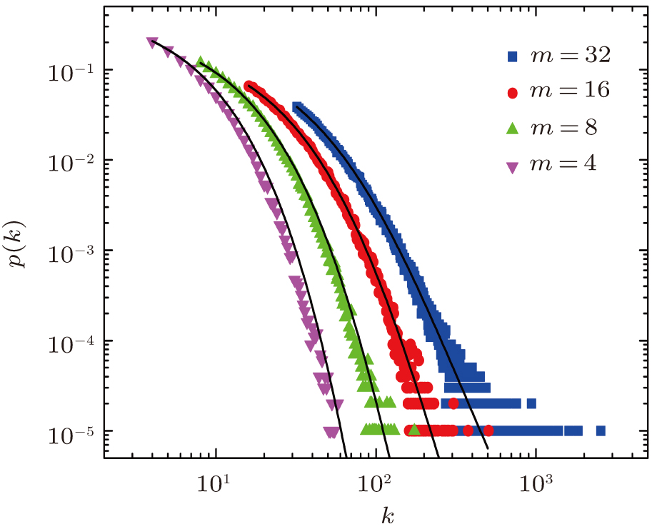
Figure 6 shows temporal behavior of γ1 − 1, which approaches a stable value with small fluctuations as soon as the network evolves. The normalization factor γ1 − 1 is 34.00(6), 20.81(5), 12.04(0), and 6.96(6) corresponding to m = 4, 8, 16, and 32, respectively. Figure 7 shows the total degree distribution obtained by simulating the model for 105 time steps, in the case of a1 = 200 and a2 = 200. As expected, one obtains general power-law distributions with the analytical exponent γ3, which equals 102.02(3), 52.04(7), 27.10(1), and 14.83(1) corresponding to m = 4, 8, 16, and 32, respectively.
4. ConclusionThe characterization and modeling of time-varying networks is of great importance in network research. A simplification of this framework is the recently proposed activity-driven network,[22] which is based on the activity potential. Like attractiveness[38] and rank,[39] the potential is a time-invariant function characterizing individual interactions. Under the assumption that memoryless agents perform uniform connections, Perra and collaborators[22] obtained the degree distribution of integrated network which is proportional to the given activity rate. In reality, however, the linking probability between individuals also displays some preference,[33] which should be considered in time-varying networks.
In this paper, we have proposed an alternative, simple and intuitive model for activity-driven networks. The present model not only allows the addition of new nodes at each time step, but also considers the state transitions between active and inactive nodes. Only the adding node can emits links to other active nodes. Both uniform and preferential transitions of nodes are considered, which yields four combinations. We have provided a general differential equation framework to study the degree distribution of nodes of integrated networks where four different schemes are formulated and compared to simulation results. Only in the case of the uniform activation and deactivation can the model show an exponential distribution of node’s degree. So long as the preference is introduced, the resulting distribution follows the power law.
The dynamic feature of the model is represented by the change in the active group of nodes. At each time step, activated nodes enter the set and deactivated ones leave, while the number of the active nodes is unchanged. Only the links between currently active nodes give rise to instantaneous dynamical interactions, such as information spreading and social contagion.[40] The addition of this feature to dynamical models may lead to more quantitative description of the dynamics on networks.


