1. IntroductionRadiative properties provide us with insight about the behavior of the matter during its interaction with a radiation field. In astrophysics and environmental science, the more specific term used for referring to radiative properties is opacity: a measure of the resistance of matter to the transmission of radiation. There are various absorption and scattering mechanisms that impede the transmission and make the material opaque to radiation, such as photo-excitation, photo-ionization, inverse bremsstrahlung, and Thomson scattering. The experimental determination of opacity relies on transmission/absorption and emission spectroscopic techniques.[1–3] However, there are many practical situations in which measurements cannot be achieved in laboratory experiments, hence theoretical predictions of opacities are inevitable.[4]
Fast and accurate calculations of radiative properties are crucial for performing radiation hydrodynamic simulations and spectroscopic diagnostics in diverse research areas, such as stellar physics, inertial and magnetic confinement fusions. While modeling such problems, average charge state and photon absorption coefficient data must be available in the wide range of density and temperature. In this regard, extensive calculations need to be performed.[5–7] A few years back, these calculations were limited because of the limited capacity of the computers, so approximate atomic physics models were developed.[8–13] Significant advances in computational techniques have taken place, so with refined numerical methods and improved computational techniques now detailed and more complex approaches to opacity calculations are possible to implement.[14–17] However, due to the fast computational speed, the average models are still used widely where detailed calculations can be compromised.[1]
In thermodynamic equilibrium, free electrons follow the Maxwell–Boltzmann distribution, whereas the energy density distribution of photons is given by the Planck distribution. Our model is based on local thermodynamic equilibrium (LTE), which implies that at any particular instant, photon and electron distributions are in equilibrium with each other. From a computational point of view, LTE simplifies the calculations because instead of solving detailed rate equations, the atomic level populations can be found by Saha and Boltzmann equations, without requiring any fundamental cross section calculations.[18]
Many computational and experimental efforts are going on in parallel for achieving reliable opacities data.[1,7,19–32] It includes a large list, but here we are giving a short introduction to some of the sources, which we have used for comparison of our results. The opacity project (OP)[33] and opacity project at Livermore (OPAL)[34] have been the early sources of opacity data for astrophysicists since the nineties, and are still used extensively for modeling various problems in stellar physics.[1] OP is an online database in which atomic data is calculated using the R-matrix method, utilizing the close-coupling approximation.[33] OPAL code calculates the solution of the Schrödinger wave equation by applying relativistic analytical potential, and level populations are found by the minimization of the system’s free energy.[34] SCO-RCG is a hybrid code and combines detailed level and statistical approaches.[35] The most recent and widely tested code in the field of stellar physics is OPAS, which is based on LTE and performs calculations by combining detailed configuration and level accounting methods.[36] STA code interpolates smoothly between detailed configuration accounting and average-atom approach.[37] CASSANDRA code utilizes a detailed configuration method for obtaining atomic data and an ab-initio method for the computation of atomic physics, employing the Dirac–Hartree–Slater approximation.[38] CORONA code obtains atomic data from Perrot’s screened hydrogenic model, and average atom model in the Thomas–Fermi approach is used for average ionization.[39] LEDCOP code uses the relativistic self-consistent Hartree–Fock method, and ionic populations are calculated by using the Saha equation.[40] THERMOS code makes use of relativistic analytical potential in solving the Schrödinger equation, and calculates occupation numbers using an average atom model.[7]
The model presented in this paper is based on the average atom approximation. At high temperature (T > 10 eV), this approximation is widely used to describe the state of matter.[41] The self-consistent potential in the average atom model is calculated for an ion with average occupation numbers of energy levels, along with the free electrons in the charge-neutral spherical cell. The cross sections for radiative properties are used in the non-relativistic limits. The atomic model is mainly adopted from Ref. [7] with the exception that we have implemented the numerical scheme of Refs. [42] and [43] for the solution of the Schrödinger equation.
This paper provides the sketch of a near-future research program as much as reporting on the first steps. Some results of our model have been reported previously[44,45] in which calculations were validated with some of the advanced codes, and the results were also tested in radiation hydrodynamic code MULTI-2D.[46] In what follows, Section 2 presents the mathematical details of the model. The numerical scheme is described in Section 3. The results are compared with the published results[47] in Section 4. Finally, Section 5 presents our conclusions.
2. Mathematical modeling2.1. Calculation of energy levels by using self-consistent potentialIn our calculations, it is assumed that a well-defined average atom can show the average behavior of all the atoms and ions at that temperature and density. This average atom is a fictitious atom with non-integral occupation numbers. It occupies a spherical cell in which a nucleus is present at the center and electrons are distributed around it following a radial distribution. The volume of the cell is defined by the mean volume per atom as
where
A is the atomic mass,

is the mass density,

is the Bohr radius, and

is Avogadro’s number. Hence the average radius

(in atomic units) is
After defining the atomic sphere, we solve the system of Hartree–Fock–Slater (HFS) equations for the self-consistent potential and wave functions. These calculations need the intra-atomic potential and distribution of electrons within the cell. We have taken these values from the Thomas–Fermi model[7] as the first guess. The HFS equations are given by
where

are energy eigenvalues and

is the HFS potential expressed as
with
ρ being the radial distribution of electrons within the cell and

the exchange potential given by
[5,7]
For the above equations to be solvable, the wave function must be separable. We have taken wave function  of the form
where

is the spherical harmonics,

are the radial wave functions, and
nlm is the set of quantum numbers defining the state of electron. The numerical procedure for calculation of

and

is taken from Ref. [
42] that solves the Schrödinger equation by piecewise exact power series expansion of radial wave functions.
[43] These series are then summed up with prescribed accuracy and the solution is obtained.
The radial electron density  is taken as a sum of the bound and free electrons
The contribution of the bound states,

, is calculated by using the radial
wave functions as
where
T is the temperature of plasma and μ is the chemical potential (both in atomic units).
The free electrons density  is calculated using the Thomas–Fermi model[7]
where

is the effective boundary of continuum, and is determined from the thermodynamic consistency condition. We have not included the effect of continuum lowering explicitly as a correction term in the equation of the energy levels, as this effect is indirectly encountered through the effective boundary of the continuum.
[12] For high temperature, a good approximation for the free electron density is

, where

is assumed to be equal to the electron density at the atomic shell boundary
where
Finally, the mean charge  can be calculated by
Equations (3)–(12) are solved in self-consistent manner.
2.2. Calculation of frequency-dependent opacityOnce the average charge state, energy levels, and occupation numbers have been determined, the total frequency-dependent opacity  is calculated as the sum of photo-excitation (bound–bound), photo-ionization (bound–free), inverse bremsstrahlung (free–free), and scattering processes as[18]
where
k denotes the cross section of the above-mentioned processes. The sum in the square brackets signifies the total cross section of the three frequency-dependent absorption processes, i.e., bound–bound, bound–free, and free–free transitions, respectively, and is corrected for the induced emission (the term in parenthesis). The scattering is taken in the classical domain where it is independent of frequency. All the coefficients are calculated using the average atom model
[13] and described in the following sections.
2.2.1. Photo-excitation coefficientPhoto-excitation coefficient  as a function of photon energy can be calculated as[48]
where

is the oscillator strength corresponding to the transition between an initial state

and a final stage

and given by
where

are the radial matrix elements between levels
k and

, and computed by the relation
The integration is carried out by using the trapezoidal rule. The method of finding

has already been described in the previous section.
The  in Eq. (15) is the line broadening profile. The best choice of the line profile that incorporates the behavior of all broadenings is the Voigt profile, which is the convolution of Lorentzian and Gaussian profiles. In our model, the Voigt profile gathers natural, Doppler, fine structure, Stark, and collisional broadenings to find out line shape function
  as
as
where
V is the Voigt function,
is the overall width of broadenings with Gaussian profile, and
is the sum of broadenings having the Lorentzian profile.
[49]The standard formulas are used for natural  and Doppler width
  ,[48] which are given by
Hydrogen-like approximation is used for both the fine structure width  [50] and Stark broadening
  , which are expressed as
Electron collisional broadening  is obtained by using the screened nuclear charge instead of the effective principal quantum numbers, and calculated as[48]
All broadening mechanisms are not equally likely, the dominance of any particular phenomenon takes place depending upon the plasma conditions.
2.2.2. Photo-ionization coefficientThe photo-ionization cross section is taken in the nonrelativistic approximation, calculated as
where

is the Thomson cross section and

is the oscillator strength for the bound-free transition given by
[5]
with

being the continuum wave functions. We have computed

using the semiclassical approximation for the central field (WKB method). The detail is given in Appendix A. 4 of Ref. [
7].
2.2.3. Inverse bremsstrahlung coefficientFor inverse bremsstrahlung coefficient, the results of hydrogen atom are used[48]
where

is the Gaunt factor and

is the degeneracy correction. The Gaunt factor

is given by
[48,51]
The degeneracy factor  is taken as[48,52]
where

is the Fermi–Dirac integral of order

.
[7] 2.2.4. Scattering coefficientAt high temperatures, the absorption cross sections for the above three processes fall to very low values, which causes a problem in numerical calculations for Rosseland mean (being the harmonic mean which diverges at very low values). Hence, scattering has to be added as the lower bound in the absorption coefficient to avoid numerical divergence.[2] Our model is currently capable of performing calculations in non relativistic limits only, so we have used Thomson scattering, which is the classical limit of Compton scattering (energy less than electron rest mass energy). It is classified as coherent scattering and given by
The contributions determined from Eqs. (14), (23), (25), and (28) are substituted in Eq. (13) to obtain the total frequency-dependent opacity (also known as extinction or attenuation coefficient).
2.3. Mean opacitiesThe radiation hydrodynamic codes require the coupling of the radiation transfer equation (RTE) with the hydrodynamic equations. The frequency-dependent opacity  appearing in RTE is a highly nonlinear function of frequency, with sudden jumps owing to the presence of ionization edges and bound–bound resonances. These sharp changes in opacity need to be tactfully handled while performing numerical calculations, as they can cause divergence at particular points. Moreover,
  calculated on a fine mesh of temperature, density, and frequency points also increases the computational cost of radiation hydrodynamic simulations. The conventional practice to simplify this situation is to replace
  with the appropriate average. Two widely used types of mean opacities are the Planck and Rosseland opacities, which are calculated by taking the weighted average of
  over the entire spectrum. The Rosseland mean opacities are of interest in optically thick plasmas, whereas the Planck mean opacities are important for optically thin plasmas. The Planck and Rosseland mean opacities in the photon energy range are defined by[53]
 | |
 | |
where

is the mass density and

is the extinction coefficient given by Eq. (
13),
T is the plasma temperature in eV and

is the Planck function expressed as
Note that the Rosseland mean opacity is calculated by taking the harmonic average of the extinction coefficient (absorption + scattering), whereas the Planck mean opacity is obtained by the arithmetic mean of the total absorption coefficient (without scattering). The numerical scheme for the calculation of the mean opacities is adopted from Ref. [54].
4. Results and discussionIn order to determine the reliability of a computer code, comparison with available cutting-edge experimental measurements is necessary. In the case of unavailability of experimental data, alternate choice becomes a comparison with state-of-the-art theoretical models and computer codes. As we are intended to show the strengths and weaknesses of our model, so the main purpose of this section is to carry out the validation of the results computed with OPAQS. We have mainly benchmarked the results of OPAQS with LEDCOP, because of its availability and extensive use in research. However, comparison is also made with many other published results, wherever possible. In what follows, we have validated our results of radial wave function, average charge state, frequency-dependent and mean opacities.
The calculations of radial wave functions ( ) are vital for the calculations of shell occupancies and oscillator strengths. The accuracy of
  guarantees the accuracy of atomic data (such as energy levels, occupation numbers, and average charge state) and opacity coefficients (bound–bound and bound–free). Figure 2 shows the results of our
  calculations for aluminium plasma at temperature of 100 eV and density of 0.27 g/cc. The independent variable
  is the dimensionless length which is scaled on the radius of the atom cell
  . It is clear that the radial part of the wave function has a strong dependence on the principle and angular momentum quantum numbers (n and l). The zeros of the function correspond to the nodes of the wave function. The number of zeros,
  , follows the relation
  , hence the 1s curve does not contain any zero, whereas the curves of 2s, 3s and 4s contain one, two, and three zeros, respectively. All the curves vanish at the center and boundary (r = 0 and
  ) of the atom cell, which shows the correct implementation of the boundary conditions. The results are compared with those in Ref. [5] and found to be in excellent agreement.
The degree of ionization is the most critical parameter in the calculations of atomic properties as it strongly influences many other plasma properties, such as pressure, conductivity, and opacity coefficients. Hence, it is a conventional practice to compare the average charge state ( ) as a necessary step while comparing different atomic models. We have validated the results of
  with the published results[47] of six extensively used computational tools, including CASSANDRA, CORONA, OPAL, THERMOS, ATMED, and LEDCOP. The calculations are performed for aluminium, germanium, and iron, which are elements of astrophysical and industrial importance. The comparison over a wide range of density and temperature is shown in Tables 1–3. It is clear that in spite of the difference in physical models and computational techniques implemented in different codes, our code shows an excellent agreement for all three elements.
Table 2.
Table 2.
 Table 2.
Comparison of average charge state for germanium plasma computed at density of 0.01 g/cc and temperatures of T = 300 eV and T = 500 eV.
.
| Code |
T = 300 eV |
T = 500 eV |
| CASSANDRA |
26.60 |
29.74 |
| CORONA |
26.90 |
29.83 |
| OPAL |
26.71 |
29.82 |
| THERMOS |
26.79 |
29.82 |
| ATMED |
26.77 |
29.82 |
| OPAQS |
26.86 |
29.82 |
| Table 2.
Comparison of average charge state for germanium plasma computed at density of 0.01 g/cc and temperatures of T = 300 eV and T = 500 eV.
. |
Table 3.
Table 3.
Table 3.
Comparison of average charge state for iron plasma computed at different densities and temperatures.
.
 (g/cc) T/eV (g/cc) T/eV |
1 |
0.0127 |
7.86 |
| 500 |
1000 |
59 |
200 |
| CASSANDRA |
22.32 |
23.91 |
12.49 |
14.68 |
| CORONA |
21.96 |
23.67 |
12.93 |
13.22 |
| OPAL |
22.53 |
23.86 |
12.79 |
13.37 |
| THERMOS |
22.35 |
23.91 |
12.79 |
14.13 |
| ATMED |
22.29 |
23.87 |
12.94 |
14.17 |
| LEDCOP |
22.68 |
23.94 |
12.83 |
14.42 |
| OPAQS |
22.41 |
23.97 |
12.89 |
14.42 |
| Table 3.
Comparison of average charge state for iron plasma computed at different densities and temperatures.
. |
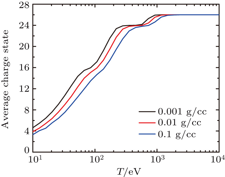
The degree of ionization helps in analyzing the overall behavior of plasma at various plasma conditions. We have tested the effect of rise in temperature on the ionization state of plasma. The computation is performed for iron plasma at three different densities of 0.001 g/cc, 0.01 g/cc, and 0.1 g/cc. The results are shown in Fig. 3. It is observed that to attain the same ionization degree, higher temperatures are required at high densities. The shell effect is clearly seen at all densities.
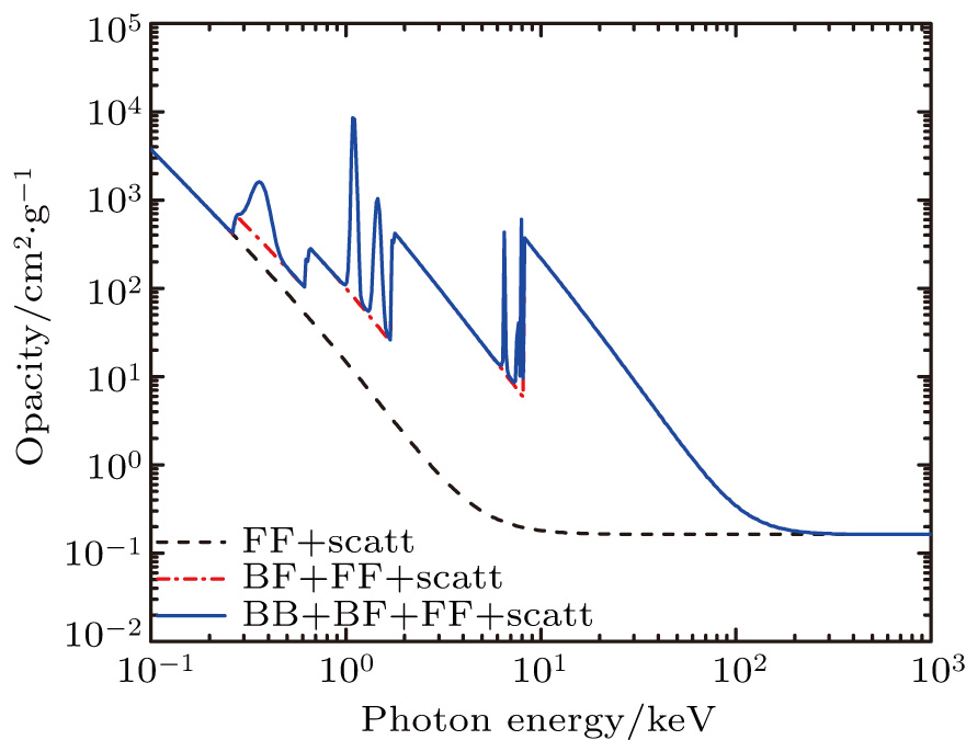
After verifying that the atomic model of OPAQS gives a correct degree of ionization, we proceed to test its calculations for radiative properties. The different contributions to opacity as a function of frequency are shown in Fig. 4 for iron plasma at  g/cc and T = 500 eV. Thomson scattering is included in all cases. The graphical trends show the behaviors of continuum opacity (bound–free + free–free + scattering) as well as total frequency-dependent opacity. The effect of eliminating the contributions of the bound–bound and bound–free transitions is also checked. It is clear that in the low photon energy range < 0.2 keV, the main contribution to opacity is from inverse bremsstrahlung (FF). In photon energy range ∼ 0.2–220 keV, the dominant mechanisms of absorption in determining the total opacity are photo-ionization (BF) and line absorption (BB). Photo-ionization edges accompanied by peaks show that various excitations are taking place along with the ionizations. At 220 keV, almost all the atoms have become fully ionized, so contributions of all the three major phenomena, bound–bound, bound–free, and free–free, cease and the only contribution left is that of Thomson scattering (Scatt), which does not depend upon the frequency. Hence, further increase in photon energy does not change the opacity anymore and we obtain a limiting value of opacity corresponding to scattering only. It is evident that plasma is almost transparent to the high-energy photons, except the minute attenuation caused by scattering.
For opacity validation, a graphical comparison between OPAQS and LEDCOP is presented in Fig. 5 for iron at density of 1 g/cc and different temperatures. It is observed that the opacity trends of OPAQS match very well with those of LEDCOP. The maxima of bound–bound transitions lie at the same energy in both cases. Finding these classical trends gives an indication of the correct implementation of the equations in the code. However, our results have few discrepancies. There is difference in the widths and heights of peaks, which could be due to choice of different line broadening mechanisms. Moreover, OPAQS has lesser number of peaks due to the fact that it is based on average atom approximation whereas LEDCOP utilizes detailed configuration approach. The small discrepancy in the bound–free part in the low-photon energy range is due to merging of photo-ionization edges with the excitation peaks.
Once the behavior of the frequency dependent opacity is tested, the next step is to validate its average behavior, i.e., the Rosseland and Planck mean opacities. The validation of the mean opacities is necessary as they serve as input parameters in radiation transfer computations. We have calculated the mean opacities for the same conditions of iron plasma and presented them in Table 4. For better comparison of atomic models, the values of the average charge state are also tabulated. The results of ATMED code are taken from Ref. [47]. Table 4 shows that the opacities computed with OPAQS are slightly higher than the others, which could be due to broader lines in its opacity trends. The reason is that opacity is mainly contributed by the lines in the absorption spectrum and broader lines tend to close opacity windows, hence increasing the resulting opacity.[21] It is also clear that the higher the temperature, the better the agreement between the obtained opacities. However, at low temperatures, OPAQS is predicting higher values, which is due to the use of the average atom approximation that serves well in the high-temperature region but appears to be slightly crude at low temperatures.[5,6] The atomic model of OPAQS is also limited in describing the energy levels compared to the models employing detailed level approach. In addition, the OPAQS model has omitted relativistic effects, LS splitting, and configuration interaction, whereas these are included in the model of LEDCOP and cause a difference in the atomic data employed in the opacity calculations.[55]
Table 4.
Table 4.
| Table 4.
Comparison of Rosseland, Planck mean opacities and average charge state for iron at density of 1 g/cc and different temperatures.
. |
Despite the good comparison of average charge state, OPAQS gives slightly higher values of opacities than those with detailed models, which is also reported elsewhere.[56] The maximum difference in Rosseland mean opacity calculation is found to be 17% at 800 eV, for Planck opacity it is 25% at 250 eV, whereas the maximum deviation in average charge state is 1.5% at 250 eV. In the literature, even the sophisticated codes have reported differences up to 300% in monochromatic opacities[36,57] and up to 60% in Rosseland mean opacities.[58] The reason for these deviations can be justified as follows. The Rosseland mean is a harmonic mean and it depends upon many factors such as features of spectrum (photo-ionization edges, line shapes, and valleys among peaks), numerical methods used in averaging, the grid points, etc. So to get an exact match among the codes or with the experimental data is indeed a challenging task for the theoretical researchers.
In Tables 5 and 6, we have presented the results of Rosseland mean opacity for aluminium and iron at density of 1 g/cc and different plasma temperatures consecutively. For aluminium plasma, the results show very good agreement with the experimental measurements (within the error bound) at temperatures of 750 eV, 1000 eV, and 1250 eV. The only exception is found at temperature of 500 eV where OPAQS is predicting a lower value. It is quite encouraging that OPAQS is in better agreement with the experiment than the rest of the codes. In contrast, the results of iron plasma show good agreement with the experimental data at temperature of 500 eV, whereas at the other three temperatures the values are slightly overestimated, yet still lie in the range predicted by the other codes.
Table 5.
Table 5.
Table 5.
Rosseland mean opacity computed for aluminium plasma at density of 1 g/cc and different temperatures. Values are taken from Ref. [47] for comparison.
.
| T/eV |
500 |
750 |
1000 |
1250 |
| TF |
40.5 |
9.09 |
2.09 |
0.83 |
| OPAL |
59.3 |
|
2.13 |
|
| HOPE |
53.1 |
|
1.92 |
|
| THERMOS |
46.1 |
10.3 |
2.14 |
0.83 |
| ATMED |
45.02 |
10.32 |
2.23 |
0.85 |
| LEDCOP |
56.84 |
|
2.19 |
0.81 |
| OPAQS |
30.75 |
10.61 |
2.55 |
0.95 |
| Experiment |
51±8 |
13±2 |
2.9±0.4 |
1.1±0.2 |
| Table 5.
Rosseland mean opacity computed for aluminium plasma at density of 1 g/cc and different temperatures. Values are taken from Ref. [47] for comparison.
. |
Table 6.
Table 6.
Table 6.
Rosseland mean opacity computed for iron plasma at 1 g/cc density and different temperatures. Values are taken from Ref. [47] for comparison.
.
| T/eV |
500 |
750 |
1000 |
1250 |
| TF |
62.5 |
7.81 |
2.70 |
1.59 |
| OPAL |
84.2 |
|
3.48 |
|
| THERMOS |
79.60 |
8.37 |
3.14 |
2.29 |
| ATMED |
86.16 |
8.59 |
2.77 |
1.77 |
| LEDCOP |
74.97 |
|
3.32 |
2.14 |
| OPAQS |
83.84 |
11.03 |
3.86 |
2.31 |
| Experiment |
82±12 |
7.8±1.0 |
2.3±0.4 |
1.3±0.2 |
| Table 6.
Rosseland mean opacity computed for iron plasma at 1 g/cc density and different temperatures. Values are taken from Ref. [47] for comparison.
. |
We have also compared the calculations of mean opacities with some other state-of-the-art opacity codes being frequently used in the field of stellar physics: STA, OP, CASSANDRA, OPAS, SCO-RCG, and LEDCOP.[59] Comparison is shown in Table 7. The results of OPAQS are tested by employing two different approaches for the broadening phenomena: Stark broadening is included in the calculations of OPAQS1, but omitted in the case study of OPAQS2. It is observed that OPAQS1 has provided good comparison of Planck mean opacities with all the other codes, whereas it has discrepancy in the calculation of Rosseland mean values, where all the results are underestimated. The values of Rosseland mean are found to improve when we reduce the effect of Stark broadening in our calculations, but in this way the values of Planck mean opacities get underestimated. The effect of other parameters is also tested by varying their values, but no other parameter is found to play such a strong role. Hence it is interpreted that the line profile is the most sensitive parameter that should be carefully tackled while performing opacity calculations. The correct choice of line broadening mechanism at given temperatures and densities is a hot topic of research nowadays.
Table 7.
Table 7.
Table 7.
Planck and Rosseland mean opacities computed for iron plasma at density of 3.4 mg/cc and different temperatures. Values are taken from Ref. [59] for comparison.
.
| T/eV |
Planck mean opacity/(cm /g) /g) |
Rosseland mean opacity/(cm /g) /g) |
| 15.3 |
27.3 |
38.5 |
15.3 |
27.3 |
38.5 |
| STA |
58650 |
33380 |
16100 |
19330 |
20500 |
7020 |
| OP |
23400 |
28000 |
14289 |
8160 |
14642 |
5978 |
| CASSANDRA |
56770 |
31250 |
16280 |
27650 |
20250 |
7545 |
| OPAS |
59441 |
36438 |
18156 |
18906 |
23323 |
8854 |
| SCO-RCG |
54652 |
30331 |
13167 |
18209 |
19335 |
6423 |
| LEDCOP |
55533 |
29263 |
15573 |
18578 |
18790 |
7359 |
| OPAQS1 |
54749 |
25208 |
14344 |
4113 |
2505 |
1687 |
| OPAQS2 |
46838 |
23452 |
13774 |
19718 |
13651 |
1306 |
| Table 7.
Planck and Rosseland mean opacities computed for iron plasma at density of 3.4 mg/cc and different temperatures. Values are taken from Ref. [59] for comparison.
. |
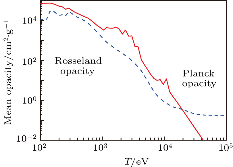
We have also tested the temperature dependence of the mean opacities, and the result is shown in Fig. 6. The calculations are performed for iron plasma at density of 0.1 g/cc and a wide range of temperatures. It is clear that both Planck and Rosseland opacities show a decreasing trend. The reason is obvious: with the increase in temperature, the average ionization of plasma increases, which means that now there are fewer number of occupied shells. The lesser number of bound levels results in decreasing the bound–bound and bound–free contributions that strongly need bound electrons for their absorption. The free–free absorption occurs in the field of ions and has very small probability at high temperatures. Thus scattering appears to be the only contributing process. The Planck mean opacity does not include the scattering term so it has a continuously decreasing trend, whereas the Rosseland mean opacity converges to a constant value corresponding to the scattering term that serves as a lower bound in this case. Thus the overall effect of increasing the temperature results in decreasing the opacity.[60] The shell effect is clearly more prominent in the case of Planck mean opacity than that of Rosseland mean opacity.[61]


