† Corresponding author. E-mail:
Porous media have a wide range of applications in production and life, as well as in science and technology. The study of flow resistance in porous media has a great effect on industrial and agricultural production. The flow resistance of fluid flow through a 20-mm glass sphere bed is studied experimentally. It is found that there is a significant deviation between the Ergun equation and the experimental data. A staggered pore-throat model is established to investigate the flow resistance in randomly packed porous media. A hypothesis is made that the particles are staggered in a regular triangle arrangement. An analytical formulation of the flow resistance in random porous media is derived. There are no empirical constants in the formulation and every parameter has a specific physical meaning. The formulation predictions are in good agreement with the experimental data. The deviation is within the range of 25%. This shows that the staggered pore-throat model is reasonable and is expected to be verified by more experiments and extended to other porous media.
The study of fluid flow in porous media has extensive engineering backgrounds[1] such as, groundwater seepage, oil and gas exploitation, thermal insulation materials, pebble-bed cooling reactors, filters, catalytic fixed bed reactors, absorbers, porous material drying, and biotechnology, among others. Investigations on porous media commonly have the perspective of flow modelling, flow resistance characteristics, transport characteristics of flow, and wall effects. Studies of porous media have a long history, going back to Darcy and Forchheimer, and can be referred to extensively in literature.[2–18] The Ergun equation is the most widely used correlation. Flow resistance through porous media is the result of frictional loss and inertia, characterized by the linear and quadratic dependence on velocity, respectively,
 |
There are two empirical constants, A and B, in the Ergun equation and the values obtained by Ergun are 150 and 1.75, respectively. Researchers[7,10,13,19–23] derived different values of A and B, as shown in Table
| Table 1.
Values of A and B in Ergun equation. . |
In the available literature, most of the efforts are towards the determination of the validity ranges of the Ergun equation. Some researchers proposed a different flow resistance formulation, as shown in Table
| Table 2.
Formulation of flow resistance. . |
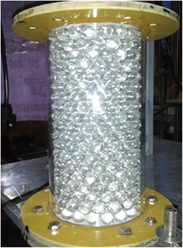
Flow resistance through a 20-mm glass sphere bed is investigated. It is found that the experimentally observed flow resistance data are much lower than the predictions of the Ergun equation. This indicates that the Ergun equation is not applicable to this situation. The staggered pore-throat model is established considering the friction loss and local loss. Moreover, a flow resistance formulation is derived.
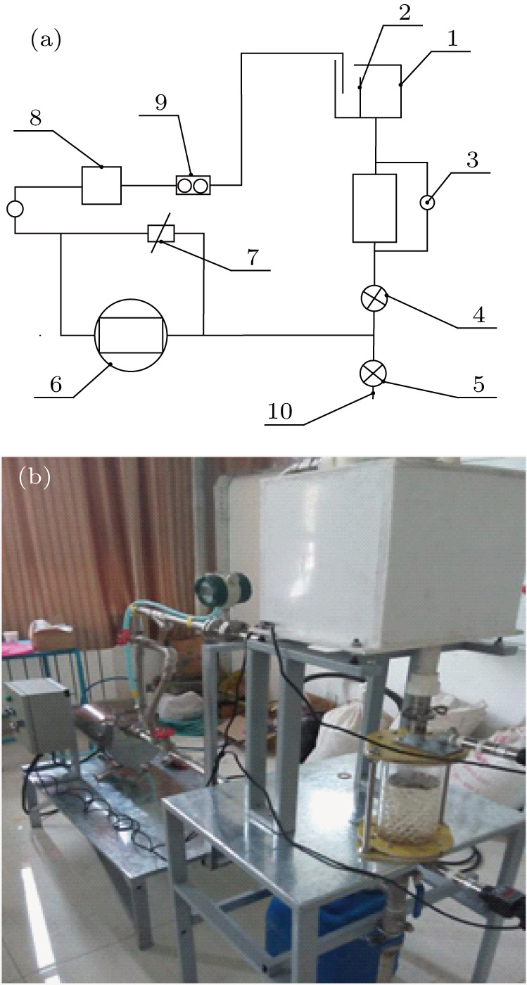
The experimental setup[27] is shown in Fig. 


The main parameters of the experiment are the flow rate and the pressure drop through the test section. They are measured by the flow meter and differential pressure meter, respectively. The differential pressure meter is of the DPG409-10WDWU type (Omega Company), with a measurement range of 0–25 mbar and an accuracy of 0.08%. The flow meter is an explosion-proof electronic flow meter of the HPLWGY-DN15 type, with a measurement range of 0.6–6 m


 |

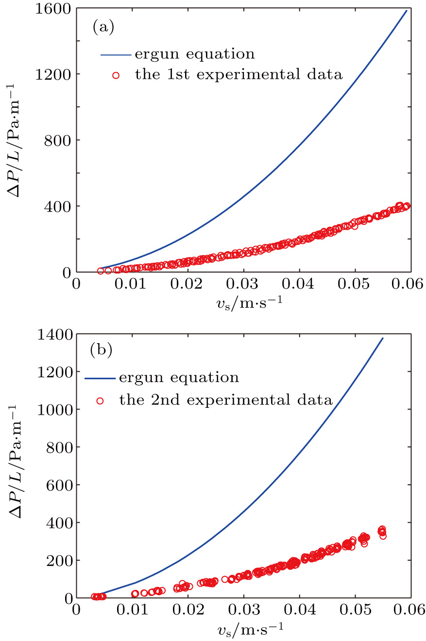
A comparison of the Ergun equation and the experimental data of the random porous media with 20 mm glass spheres is shown in Fig.
There is a big gap between the experimental data and the Ergun equation, as seen in Fig.
The original pore-throat model proposed by Yu and Wu[18] shows that porous media are aligned by equivalent diameter particles. A periodic unit consists of four adjacent particles. However, natural porous media are in fact more randomly staggered. Glass spheres are closer to a staggered arrangement based on the random packing of the test section. Regarding the three adjacent particles as a unit seems more reasonable. The staggered pore-throat model is established as shown in Fig. porous media are packed randomly by spherical particles with equivalent particle diameter the particles of porous media are staggered in a regular triangle arrangement; the velocity of the fluid in porous media is the average velocity; fluid flows from one inlet and flows out from two outlets, where the radius of each outlet is half that of the inlet.

 | Fig. 4. Staggered pore-throat model and its geometry parameters. (a) Staggered pore-throat model. (b) The geometry parameters of the pore-throat. |
The particles in porous media are in a regular triangle arrangement. 


The area of the particle A is
 |
The unit area, which is the area of the rectangle 
 |

 |
The distance between the particles is determined by solving Eqs. (
 |
 |
The pore-throat ratio β is
 |
The pressure drop through the unit is characterised as the flow resistance, which is the sum of the friction resistance and the local resistance, which are calculated below. The fluid channel is considered to be a tortuous capillary, and the pressure drop is the friction resistance loss of the circular pipe. The friction loss is
 |


Nikuradse[28] indicates that the friction resistance coefficient is only related to the Reynolds number in the laminar flow. It is irrelevant to the relative roughness. The friction resistance coefficient is 
The Reynolds number 
 |
The friction resistance loss is
 |
The diameter of the channel 
 |
The friction loss per unit length is obtained by substituting
 |
The tortuosity 
 |
The local loss is the sum of one sudden expansion local loss and two sudden contraction local losses. The sudden expansion local resistance coefficient 

 |


 |
Therefore, the total local resistance coefficient 
 |
Each local resistance is calculated twice, considering that the inlet of this unit is the outlet of the former unit and the outlet of this unit is the inlet of the next unit. The local resistance loss coefficient should therefore be multiplied by 0.5 personally. Then, the modified local resistance loss coefficient is
 |
The local resistance is
 |
The local resistance per unit length is obtained by substituting 
 |
The total flow resistance is
 |
The dimensionless form of the flow resistance is
 |
The dimensionless form of the Ergun equation is
 |
Comparison of the experimental data and the model prediction is shown in Fig.
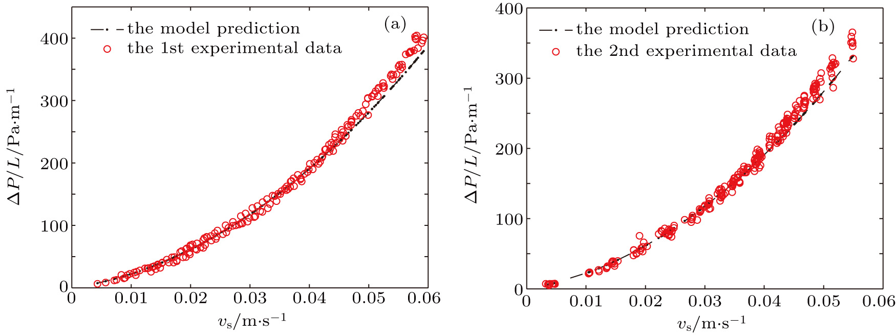 | Fig. 5. (color online) Comparison of the predicted value of the model to the (a) first experimental data and (b) second experimental data. |
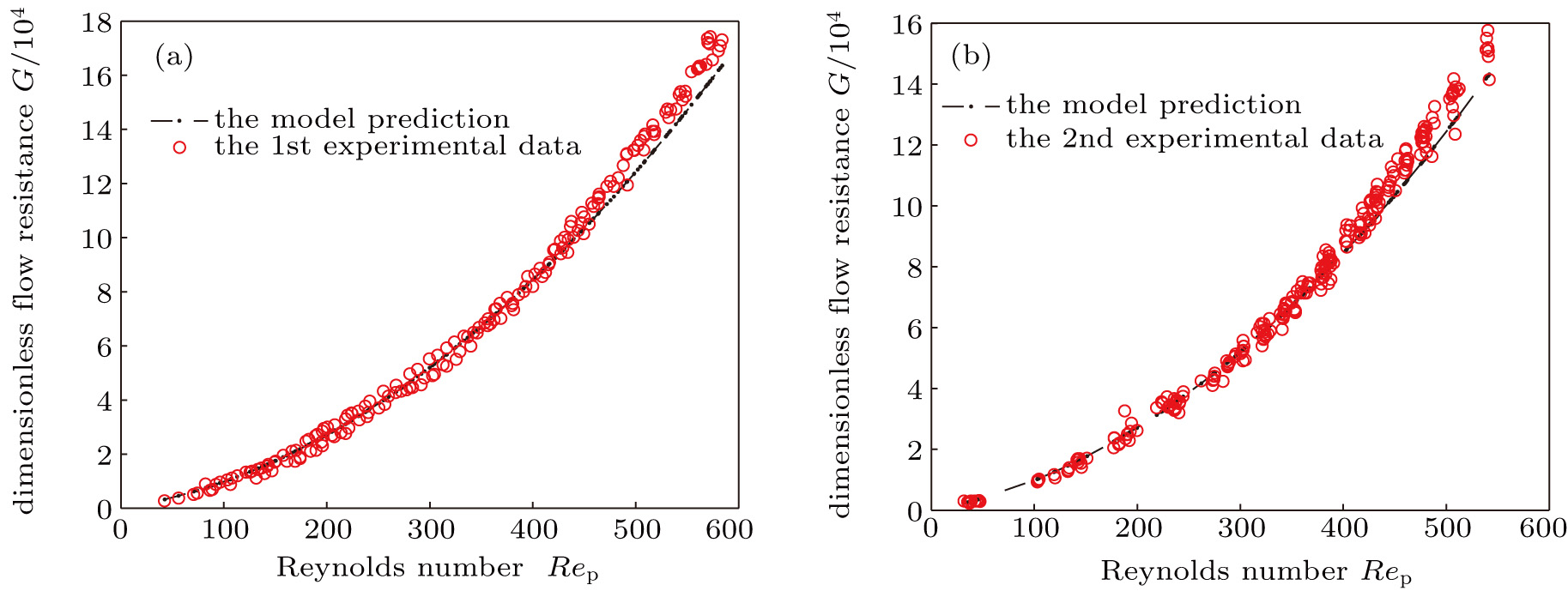 | Fig. 6. (color online) Comparison of the dimensionless predicted value of the model to (a) first experimental data and (b) second experimental data. |
The staggered pore-throat model predictions are in good agreement with the experimental data, as seen in Figs.
However, the errors between the model prediction and the experimental data must still be compared, as shown in Table
| Table 3.
Comparison of the error between the model prediction and the experimental data. . |
If the distance between the local resistances is appropriate, and the correction factor is 2.5 instead of 0.5 in Eq. (
| [1] | |
| [2] | |
| [3] | |
| [4] | |
| [5] | |
| [6] | |
| [7] | |
| [8] | |
| [9] | |
| [10] | |
| [11] | |
| [12] | |
| [13] | |
| [14] | |
| [15] | |
| [16] | |
| [17] | |
| [18] | |
| [19] | |
| [20] | |
| [21] | |
| [22] | |
| [23] | |
| [24] | |
| [25] | |
| [26] | |
| [27] | |
| [28] | |
| [29] |


