A damping boundary condition for atomistic-continuum coupling
Zhang Jie1, Tieu Kiet1, †, Michal Guillaume1, Zhu Hongtao1, Zhang Liang1, Su Lihong1, Deng Guanyu1, 2, Wang Hui1
School of Mechanical, Materials, and Mechatronic Engineering, University of Wollongong, Wollongong, NSW 2522, Australia
Department of Materials Science and Engineering, Kyoto University, Kyoto 606-8501, Japan


† Corresponding author. E-mail: ktieu@uow.edu.au

Abstract

The minimization of spurious wave reflection is a challenge in multiscale coupling due to the difference of spatial resolution between atomistic and continuum regions. In this study, a new damping condition is presented for eliminating spurious wave reflection at the interface between atomistic and continuum regions. This damping method starts by a coarse–fine decomposition of the atomic velocity based on the bridging scale method. The fine scale velocity of the atoms in the damping region is reduced by applying nonlinear damping coefficients. The effectiveness of this damping method is verified by one- and two- dimensional simulations.

1. Introduction

Atomistic simulation is applied widely to study mechanics and materials at the nanoscale.[1] In spite of rapid development in computer techniques, atomistic simulation still suffers from limitations in terms of spatial and temporal scales. On the other hand, the continuum method is not capable of describing accurately physical phenomena at the atomic level, despite its efficiency.[2,3] Therefore, the multiscale method is proposed to overcome the limitations of those existing simulation tools, such as molecular dynamics (MD) and finite element method (FEM), so that complex phenomena at a small scale can be explored without sacrificing too much computational time. During the past decades, many multiscale methods have been developed, including concurrent coupling of length scales (CLS),[4] bridging scale method (BSM),[57] bridging domain method (BDM),[8] and hybrid simulation method (HSM).[9] They have been successfully used for a wide range of areas, such as nanoindentation,[10,11] crack,[12,13] and nanotribology.[1416]

One major difficulty in multiscale coupling is that the high frequency or the short wavelength components of waves from the atomistic region cannot be captured by coarse continuum mesh. Those components that fail to propagate appropriately into the continuum region are reflected back into the atomistic region at the atomistic/continuum interface, resulting in a spurious increase of temperature. This phenomenon is known as spurious wave reflection,[17] which can generate considerable numerical errors. Recently, several multiscale techniques have been applied to handle the spurious wave reflection with varying degree of effectiveness. Cai and coworkers[18] proposed a time-dependent boundary condition to minimize elastic wave reflection based on a generalized Langevin equation, and applied to one-dimensional (1D) problems. The method requires a numerical calculation of response functions, which could be time-consuming for multiple dimensions. Wagner and Liu[5] developed a so-called bridging scale method (BSM) in which the displacement is decomposed into the coarse and fine scales by using a projection operator. They eliminated unwanted reflections by analytically accounting for high-frequency components of waves as an additional force term in the standard MD equation. However, the implementation of the BSM is not straightforward as both Fourier and Laplace transforms are needed as well as the storage of the boundary atom displacement history. Sadeghirad and Liu[19] added a viscous term into the motion equation of MD in order to reduce the non-physical reflections at the MD/FEM interface. Their damping algorithm performed well in the frameworks of BSM and BDM. Other effective methods have been developed so far, including non-reflection interfaces by E and Huang,[20] ‘stadium’ damping method by Qu et al.,[21] spatial filters by Ramisetti et al.[22]

In this study, a new damping boundary condition is proposed to remove the spurious wave reflection that occurs in atomistic-continuum coupling. In this method, firstly, we use a projection operator proposed by Wagner and Liu[5] to separate the total velocity of each atom within the overlapping subdomain of atomistic and continuum domains into coarse and fine components. The coarse velocities of the atoms are not modified so all data of mechanical deformation can be propagated into a continuum region. On the other hand to reduce the spurious reflections the fine velocities are eliminated by applying the damping coefficients. One key result in this paper is that the damping coefficients ramp nonlinearly over the width of the overlapping domain. The method is implemented by a multiple-time-step algorithm. The good performance of the proposed method is verified by one- and two- dimensional problems.

2. Presentation of the method

Figure 1 shows the one-dimensional model for the presented damping method. This model consists of three regions: the FEM region, the MD region, and the damping region (dashed line).

Fig. 1. Schematic diagram of one-dimensional multiscale coupling between FEM and MD with a damping region.

We start by a brief introduction of the coarse-fine decomposition following Wagner and Liu’s work[5] in Subsection 2.1. The coarse–fine decomposition is applied to the velocities of the atoms within the damping region where the FEM and MD regions overlap. Nonlinear damping coefficients used to reduce the fine parts of the atomic velocity are calculated for all atoms in the damping region in Subsection 2.2. The ghost atom (dotted circle) is used to provide a physical boundary condition for the MD region.[23] It follows the movement of the mesh in the FEM region. The movement of atoms (filled circles) and nodes (open circles) in the FEM and MD regions are governed by the standard MD and FEM equations, which will be given in detail coupled with a multiple-time-step algorithm in Subsection 2.3.

2.1. Coarse–fine decomposition in the damping region

According to the original bridging scale method (BSM),[5] the total displacement of an atom α in the damping region consists of a coarse scale and a fine scale as given in Eq. (1).

As the coarse scale is the projection of the total scale on the FEM space of displacement, it can be defined as

where is the shape function of the initial position of the atom α at node I, and is the displacement of node I. The fine scale describes the components of the total displacement that cannot be represented by the coarse scale. The fine scale is defined as the difference between the total scale and the coarse scale . A projection operator is obtained by solving minimizing the sum of the square of the difference between the coarse and the total scale as given in Eq. (3)

Solving Eq. (3) with respect to yields

Multiplying to both sides of Eq. (4) yields

The projection matrix is defined as

Therefore, the coarse scale is the least-square fit of the total scale. The fine scale is obtained by subtracting the coarse scale from the total scale as given in Eq. (7)

where is the identity matrix. The derivative of Eq. (7) with respect to time gives
where and are the velocity vectors of the total and fine scales, respectively. Similarly, the velocity vector of the coarse scale can be written as

Finally, the equation of the total velocity for the atoms in the damping region can be written as

where is the nodal velocity vector. As given by Eqs. (5)–(7), the projection matrix is used to decompose the total velocity of the atoms in the damping region into the coarse and fine scales at each time step. Note that the projection matrix depends on the initial geometry of the model, and is only needed to be calculated once before running simulations.

2.2. Calculation of damping coefficient

After the coarse–fine decomposition of the velocities for the atoms in the damping region, the fine velocities are rescaled by multiplying the vector of the damping coefficients θ, while the coarse parts are not changed. Therefore, the atomic equation of the total velocity with θ can be written as

Each element of the vector θ corresponds to the damping coefficient of each atom in the damping region. For the model in Fig. 1, the damping coefficient of one atom α in the damping region is defined as

where is the position of atom α, is the left boundary of the FEM region, W is the width of the damping region, s is the parameter between 0 and 1. If s = 0, as all elements of θ equal 1, there is no damping effect on the fine scale. If s = 1, the elements of θ ramp linearly over the width of the damping region, which is similar to the damping condition in Qu’s work.[21] If , the elements of θ vary nonlinearly. Both linear and nonlinear damping conditions can ensure a gradual change of the atom dynamics from the MD region to the damping region. As demonstrated in Section 3 however, the nonlinear coefficients show a better performance for reducing the spurious wave reflections compared to the linear ones.

2.3. Multiple-time-step algorithm

In the damping region, the continuum mesh is not refined down to the atomistic level when using the damping method. This allows a larger time step used in the FEM region compared to that in the MD region, and saves the computation time. A multiple-time-step algorithm is proposed as follows. We define the MD time step and the FEM time step as and , respectively. As the FEM model is advanced one time step , the MD model is advanced by m steps of . The movement of the atoms, in both MD and damping regions is updated by using an explicit central difference method as given in Eqs. (13)–(15). Other methods, such as velocity verlet method,[1] can also be used.

where is the atomic acceleration vector, is the atomic force vector which is the first derivative of the interatomic potential, is a diagonal matrix with diagonal elements equal to atomic masses, and .

In each MD time step, the fine velocities of the atoms in the damping region are obtained according to Eq. (8), and rescaled by multiplying the damping coefficient in Eq. (12). Then, the total velocities of those atoms are recalculated according to Eq. (11).

After the quantities , , and of the atoms in the MD and damping regions are obtained, the nodal movement in the FEM region is updated from n to n + 1 by using the explicit central difference method as given in Eqs. (16)–(18).

where is the nodal acceleration vector. and are the lumped mass matrix and the internal force vector of the FEM region, respectively. The internal force is calculated based on the Cauchy–Born (CB) rule, which is widely used in the multiscale simulations.[5,8,23,24] The continuum stress can be directly calculated from the interatomic potential using the CB rule. Details about the CB rule and its applications can be found in the quasicontinuum method[23] and the review paper by Park et al.[7] Instead of Eqs. (16)–(18), the displacement and velocity of the boundary node in the damping region, e.g., the leftmost node of 1D model in Fig. 1, are determined by weighted averaging the corresponding quantities of the atoms at time step n + 1 based on the hybrid simulation method (HSM) proposed by Luan and Robbins.[9] Therefore, the displacement and velocity are given as
where and are the displacement and velocity vectors of the atoms whose initial positions are close to the boundary node with a distance r less than a given distance . is the weight vector of those atoms. Each element of is calculated by a weighing function,[25] which is given in Eq. (13).

The given distance is comparable to the size of one finite element.[9] The weighted averaging method from Eqs. (19) and (20) is used to transmit atomic information to the FEM region. Meanwhile, the transmission of FEM information to the MD region is achieved by interpolating the displacement of the ghost atom at time step n + 1 shown in Eq. (22)

where and are the shape function and the displacement of the nodes that form an element containing the ghost atom, respectively.

3. One-dimensional example
3.1. Model set-up

In the one-dimensional example, we apply the damping method proposed in Section 2 to a wave-propagation problem similar to those used in Refs. [5] and [8]. The Lennard-Jones (LJ) potential is used to describe the interatomic interactions. This potential is expressed as

where ε and σ are characteristic energy and length scales, respectively. We use ε = 0.2 eV and σ = 0.11 nm, so the equilibrium bond length is . As the nearest-neighbor interactions are considered, the cut-off radius of the LJ potential is . As mentioned above, the constitutive law of the FEM model is governed by the Cauchy–Born rule. Thus, the first Piola–Kirchhoff stress in the FEM region is obtained as
where is the deformation gradient of an FEM element, and is the potential energy density obtained from the LJ potential.

The entire region consists of 271 atoms in total, 35 atoms in the damping region, and 42 linear elements of equal size in the FEM region. The MD time step is ps. The FEM time step is 10 times larger than . The initial displacements of the atoms are expressed as

where A = 0.0015 nm, μ = 50r0, b = 0.1, , , and . The prescribed displacement at time t = 0 is plotted in Fig. 2. The initial velocities of the atoms and the nodes at time t = 0 are zero.

Fig. 2. (color online) The initial displacements of the one-dimensional example.
3.2. Results and discussion

In the damping method of this study, the parameter s has a crucial effect on the reduction of the spurious wave reflections. An a priori test is used to determine the optimal parameter s.

We choose four different values of ) for nonlinear damping. Meanwhile, s = 0 and s = 1 are the parameters of non-damping and linear damping, respectively. Figure 3 shows that the initial wave is propagated into the FEM region at time t = 9 ps with the spurious reflections of varying degree. Without any damping treatment (s = 0), the majority of the high frequency components of the wave are reflected into the MD region as shown in Fig. 3(a). Comparing with the results in Fig. 3(a), both the nonlinear damping methods in Figs. 3(b)3(e) and the linear damping methods in Fig. 3(f) can dramatically reduce the wave reflections. More importantly, the nonlinear damping method with the parameters s = 0.01, 0.05, and 0.1 shows a better performance than the linear damping method. To make a clearer comparison for different damping conditions, a time history of the energy in the MD region has also been plotted in Fig. 4. The energy in the MD region is the sum of the kinetic and potential energy of the atoms, and is normalized by the initial potential energy due to the prescribed displacement.

Fig. 3. (color online) Snapshot of displacement at t = 9 ps for different parameter s. (a) s = 0; (b) s = 0.01; (c) s = 0.05; (d) s = 0.1; (e) s = 0.5; (f) s = 1. Blue squares and red circles indicate the atoms and the nodes, respectively.
Fig. 4. (color online) Normalized energy of the MD region as a function of time for different parameter s.

As shown in Fig. 4, 74.9% of the energy remains in the MD region for s = 0. The rest of the energy is 8% of the total when the linear damping method is used. Figure 4 shows that the remaining energy using the nonlinear damping method for four different values of s is lower than that using the linear damping one (s = 1). The optimal value of s is 0.05, which results in 0.7% of the remaining energy. Without further mention, the nonlinear damping parameter is 0.05 for the following cases.

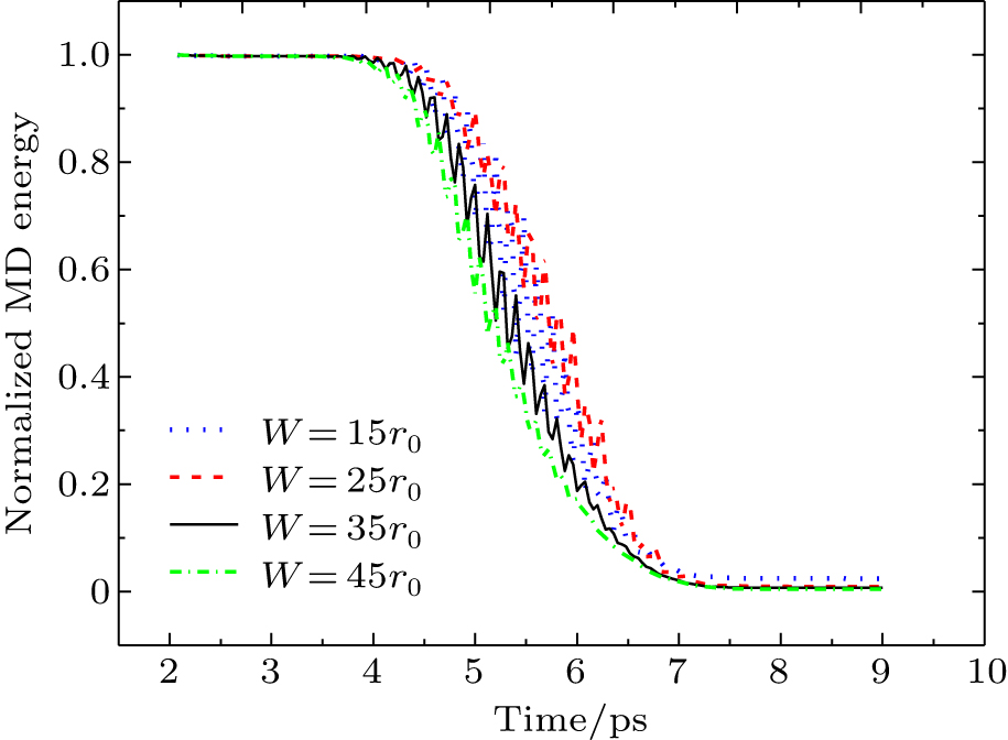
Similar to the bridging domain method,[8] the width of the damping region in our method also plays a role in the reduction of spurious wave reflections. As the width increases, the remaining energy in the MD region reduces as shown in Fig. 5. The normalized energy decreases from 2.4% to 0.4% when the width of the damping region increases from to . When the width is larger than , the energy that remains in the MD region is less than of the total energy. Moreover, the larger damping region for the model requires more computational time. Therefore, the width is used as a compromise between the effects on the reduction of wave reflection and the computation time.

Fig. 5. (color online) Normalized energy of the MD region as a function of time with different widths of the damping region.

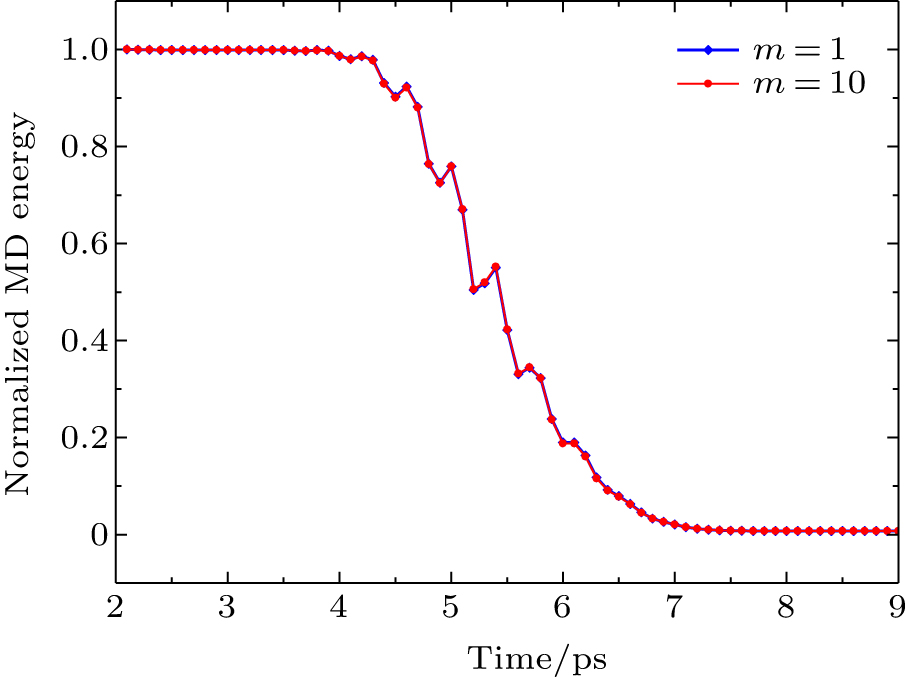
In Fig. 6, the time history of the normalized energy in the MD region from two different ratios between the FEM time step and the MD time step is compared. Their results are almost identical as shown in the figure, indicating that our multiple-time-step algorithm in Subsection 2.3 is stable and accurate. The multiple-time-step algorithm used here can ensure that both the FEM and MD models are run at different time steps with appropriate sizes. More importantly, it can avoid a time-wasting situation that the FEM time step is limited to the time step at the atomic level.

Fig. 6. (color online) Normalized energy of the MD region as a function of time with and .

In Fig. 7, the model using the nonlinear damping method is benchmarked by a full MD model. The full MD model consists of 646 atoms. At t = 9 ps, the wave in the FEM region of the multiscale model is similar to that in the full MD model. As the high frequency components of the wave in the multiscale model are eliminated, there are some deviations between their amplitudes.

Fig. 7. (color online) Snapshot of displacement at ps for full MD and the nonlinear damping method.

Figure 8 shows snapshots of displacement at t = 9 ps for the bridging scale method (BSM) and the nonlinear damping method, respectively. The geometries of the two models are the same. According to the bridging scale method,[7] two terms that account mathematically for the effects of the fine scale in the FEM region are added into the movement equation of the boundary atom (in this study, it is the atom next to the ghost atom) as given in Eq. (26)

where and are the acceleration of the boundary atom and the force on it, respectively. is the time history of the fine scale displacement for the boundary atom. is the time history kernel (THK), serving as an exit for the fine scale energy from the MD region. For the one-dimensional case here, the expression of the THK is shown in Eq. (18).
where k and ω are the stiffness and the natural frequency of the atomistic bond, respectively. is the first order Bessel function. The THK as a function of time t is plotted in Fig. 9 On a purpose of clearly showing, the time in the figure only reaches 2 ps. As shown in Fig. 9, the first several oscillations of contribute mainly to the second term on the right-hand of Eq. (26), as the amplitude decays quickly after 0.5 ps. In two- and three-dimensional cases, the THK is usually truncated for saving computational time. Park et al.[7,12,26] have discussed the effect of the truncation on the results.

Fig. 8. (color online) Snapshot of displacement at t = 9 ps for the bridging scale method (BSM)[7] and the nonlinear damping method.
Fig. 9. Plot of time history kernel as a function time.

in Eq. (26) is the random force, which is zero in this study. It can be seen that the results from our method and the BSM are quite close in Fig. 8. Meanwhile, the remaining energy in the MD region for our method and the BSM is 0.7% and 0.02%, respectively. Although the BSM performs a little better on the reduction of the spurious wave reflections, it is usually difficult to calculate the THK, especially in two- and three- dimensional cases.[12,26] Moreover, in our method, storing the time history information for the boundary atom is not needed.

4. Two-dimensional (2D) example
4.1. Model set-up

The extension of our damping method to two and three dimensions is straightforward. In this section, we apply the damping method to the pulse propagation problem, which was previously studied by Luan and Robbins using the hybrid simulation method (HSM).[9]

Figure 10 shows the geometry of two-dimensional pulse propagation. The atomistic interactions in the MD region are described by the LJ potential with the parameters ε = 0.15 eV and σ = 0.3 nm. The atoms sit on the triangular lattices with the equilibrium bond length . The cutoff radius of the LJ potential is . The FEM region is equally divided by the three-node elements with a minimum edge length of . Similar to the one-dimensional example, the Cauchy–Born rule is used to describe the constitutive law. The coupling scheme of the HSM is based on Eqs. (19)–(22) as given in Section 2.3, or in Luan and Robbins’ work.[9,14] The displacement of each boundary node in the damping region is obtained by averaging the displacements of the atoms within a circle with the radius of and centered at that node.

Fig. 10. (color online) Geometry of two-dimensional pulse propagation. Blue filled circles indicate a shear layer of the atoms while red filled circles indicate the free atoms. Open circles indicate the ghost atoms.

Periodic boundary conditions are applied for both MD and FEM regions along the x direction. The right boundary of the FEM region is fixed in Fig. 10. Following Luan and Robbins’s work,[9] the shear layer (blue circles) in Fig. 10 is forced to move along the x direction according to the form of the displacement , where and . The movement of the shear layer can generate a pulse with the width , which propagates from MD to FEM. Full MD simulations are also conducted for comparisons.

4.2. Results and discussion

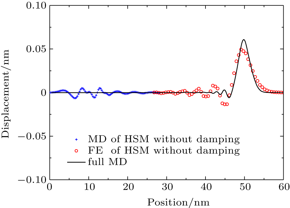
Figure 11 shows the shear displacement as a function of position along the y direction. The shear displacement is extracted from the central line of the model when the leading edge of the pulse reaches the rightmost boundary. Due to different dispersion relations, there are different oscillations at the tail of the pulse in the full MD and the HSM. Similar results were also presented by Luan and Robbins.[9] In this study, however, we focus on spurious reflections at the MD/FEM interface. In Fig. 11, noticeable reflections can be observed in the MD region. This is due to the resolution change between MD and FEM. Those reflections could lead to both an increase of the kinetic energy with time and the system instability.

Fig. 11. (color online) Displacement along x as a function of position along y at the time when the leading edge of the pulse reaches the rightmost boundary for both the non-damping HSM and full MD simulations.

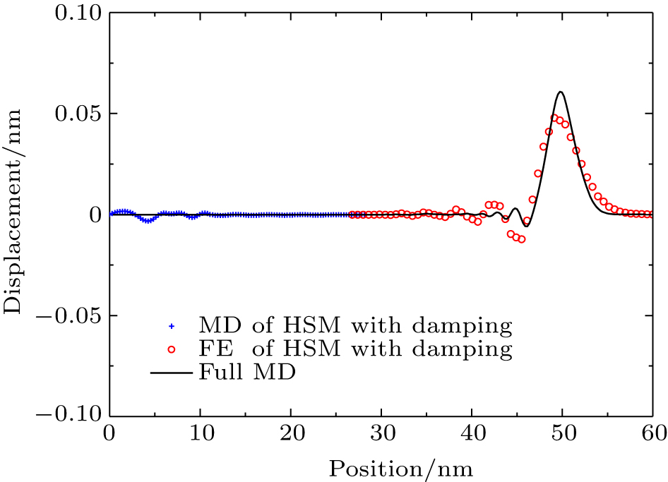
Similar to the one-dimensional example in Section 3, we apply the nonlinear damping method with the damping parameter s = 0.05 to the HSM. As shown in Fig. 12, the spurious reflections reduce significantly. To show quantitatively the performance of the damping method, the ratio between the energy of the reflected wave and the total energy of the initial pulse is also calculated. The reflected energy without damping is 15.7% while it decreases to 1.7% with the nonlinear damping. Larger damping regions have also been tested. The reflected energies are 0.75% and 0.44% corresponding to 4.2 nm and 5.4 nm of the damping lengths along the y direction, respectively. The results of the two-dimensional example indicate that our damping method is capable of handling more realistic problems.

Fig. 12. (color online) Displacement along x as a function of position along y at the time when the leading edge of the pulse reaches the rightmost boundary for both the damping HSM and full MD simulations.
5. Conclusion and perspectives

In this study, a nonlinear damping method is proposed for the reduction of the spurious wave reflection in the atomistic-continuum coupling. The damping method is based on a coarse-fine decomposition, and is performed by a stable multiple-time-step algorithm. Its effectiveness is verified by one- and two-dimensional examples with measures of displacement and MD energy. The results show that this damping method has a better performance compared to the linear damping method. Its effects on reducing the spurious wave reflections are comparable to the THK in the bridging scale method, but its implementation is more straightforward. The successes in two-dimensional cases indicate that the nonlinear damping method is practical and not limited to one dimension. The extension of our method to three dimensions will be carried out in the future.

Reference
[1] Rapaport D C 1995 The art of molecular dynamics simulation New York Cambridge University Press 60 62
[2] Deng G Y Tieu A K Si L Y Su L H Lu C Wang H Liu M Zhu H T Liu X H 2014 Comput. Mater. Sci. 81 2
[3] Deng G Y Lu C Su L H Tieu A K Yu H L Liu X H 2013 Comput. Mater. Sci. 74 75
[4] Broughton J Q Abraham F F Bernstein N Kaxiras E 1999 Phys. Rev. 60 2391
[5] Wagner G J Liu W K 2003 J. Comput. Phys. 190 249
[6] Tang S Hou T Y Liu W K 2006 Int. J. Numer. Method Eng. 65 1688
[7] Park H S Liu W K 2004 Comput Methods Appl. Mech. Eng. 193 1733
[8] Xiao S Belytschko T 2004 Comput Methods Appl. Mech. Eng. 193 1645
[9] Luan B Hyun S Molinari J F Bernstein N Robbins M O 2006 Phys. Rev. 74 046710
[10] Tadmor E B Miller R E Phillips R Ortiz M 1999 J. Mater. Res. 14 2233
[11] Ren G Zhang D Gong X 2011 Phys. Lett. 375 953
[12] Park H S Karpov E G Liu W K Klein P A 2005 Philos. Mag. 85 79
[13] Ren G Tang T 2014 Chin. Phys. 23 118704
[14] Luan B Robbins M O 2009 Tribol. Lett. 36 1
[15] Anciaux G Molinari J F 2010 Int. J. Numer. Method Eng. 83 1255
[16] Michal G Lu C Kiet Tieu A 2014 Comput. Mater. Sci. 81 98
[17] Adelman S A Doll J D 1974 J. Chem. Phys. 61 4246
[18] Cai W Koning M Bulatov V V Yip S 2000 Phys. Rev. Lett. 85 3213
[19] Sadeghirad A Tabarraei A 2013 Comput. Mech. 52 535
[20] E W Huang Z 2001 Phys. Rev. Lett. 87 135501
[21] Qu S Shastry V Curtin W A Miller R E 2005 Model. Simul. Mater. Sci. 13 1101
[22] Ramisetti S B Anciaux G Molinari J F 2013 Comput Methods Appl. Mech. Eng. 253 28
[23] Tadmor E B Ortiz M Phillips R 1996 Philos. Mag. 73 1529
[24] Anciaux G Molinari J F 2009 Int. J. Numer. Method Eng. 79 1041
[25] Miller R E Tadmor E B 2009 Model. Simul. Mater. Sci. 17 053001
[26] Park H S Karpov E G Klein P A Liu W K 2005 J. Comput. Phys. 207 588