Quantum-mathematical model of edge and peak point in Fresnel diffraction through a slit
Luo Xiao-He, Mei Hui, Zhu Qiu-Dong, Wang Shan-Shan, Hou Yin-Long
Beijing Key Laboratory of Precision Photoelectric Measuring Instrument and Technology, School of Optoelectronics, Beijing Institute of Technology, Beijing 100081, China


† Corresponding author. E-mail: huim@bit.edu.cn

Abstract

The intensity distribution in Fresnel diffraction through a slit includes numerous small fluctuations referred to as ripples. These ripples make the modelling of the intensity distribution complicated. In this study, we examine the characteristics of the Fresnel diffraction intensity distribution to deduce the rule for the peak position and then propose two types of quantum-mathematical models to obtain the distance between the edge and the peak point. The analysis and simulation indicate that the error in the models is below . The models can also be used to detect the edges of a diffraction object, and we conduct several experiments to measure the slit width. The experimental results reveal that the repetition accuracy of the method can reach .

1. Introduction

Diffraction by a slit is a widely known phenomenon and has been observed in many fields, such as x-rays,[14] profile parameter measurement,[5,6] and metallic film measurement.[7] Analyses of this phenomenon, thus far, are mainly focused on far-field Fraunhofer diffraction[810] and near-field Fresnel diffraction by a single edge, because their intensity distributions are simple. In contrast, the present study reveals that the Fresnel diffraction by a slit has a considerably more complex intensity distribution.

A number of studies have described the calculation of the Fresnel diffraction intensity pattern.[1118] Extreme points of the intensity pattern are used in many applications of Fresnel diffraction. For example, reference [19] makes use of the technique of locating the minimum to measure large-size parallelism, and reference [12] uses the expression of the location of extreme points to describe the focal effect of Fresnel diffraction by a slit.

In Fresnel diffraction, the shape of the diffraction object and the diffraction pattern exhibit a fair degree of similarity. On this basis, we expect that the relation between the edge and some feature points of the intensity pattern could be used to measure the profile of the diffraction object. The peak with the strongest signal in the pattern is used as the feature point. Figure 1 presents the Fresnel diffraction intensity pattern by a slit, where a is the slit width, d is the diffraction distance between the slit plane and the receiving plane, and both the slit plane and the receiving plane are perpendicular to the incident plane wave.
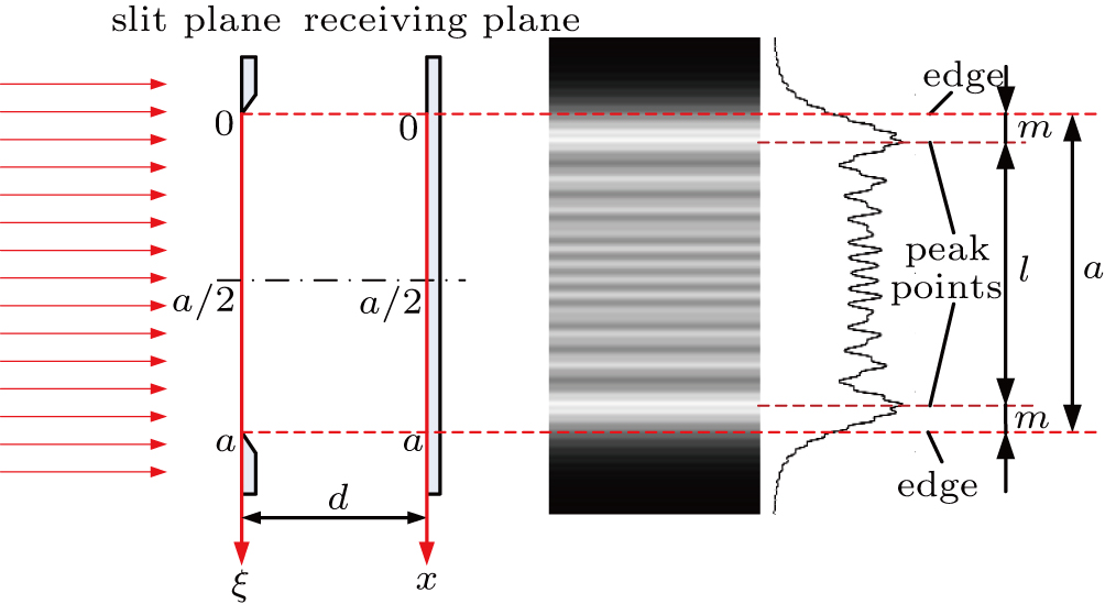
Fig. 1. (color online) Coordinate system and intensity pattern of the Fresnel diffraction by a slit with λ = 650 nm, a = 3 mm, and d = 300 mm.

If the distance l between the two peak points and the accurate distance m between the edge and the peak points are determined, then the two edges of the slit can be located, and the slit width a can be measured using the formula . Evidently, the error in measurement is affected by the accuracy of m. The expression for m has been presented in Ref. [12] and is the same as that of the Fresnel diffraction by a single edge without considering the interaction of the two slit edges. In fact, the interaction of the two slit edges results in small fluctuations in the intensity distribution. These fluctuations are referred to as ripples, and these ripples make the expression for m in Ref. [12] less accurate. This paper proposed two types of modified expressions of m in different forms.

In Fig. 1, the slit has two edges located at ξ = 0 and ξ = a, the projections of the two edges on the receiving plane are located at x = 0 and x = a. The Fresnel pattern is symmetric to x = a/2. Therefore, in this paper, we only take the edge located at ξ = 0 as the target to detect the corresponding peak position; thus, the value of m (distance between the peak point and the edge) equals the coordinate value of the peak point.

All the equations in this paper are based on the coordinate system shown in Fig. 1.

2. Fresnel diffraction pattern

According to the analysis by Southwell,[20] the Fresnel approximation for collimated propagation is sufficiently accurate for a large scope of (where λ is the wavelength, d is the diffraction distance, and a is the slit width), and the aforementioned scope includes this paper.

In this paper, we consider that the models for the Fresnel diffraction by a slit and a single edge are similar; therefore, we discuss the Fresnel diffraction model by a slit based on that with a single edge.

2.1. Probability intensity distribution

From Ref. [21], the expression for the Fresnel integral is

where α is the argument of the Fresnel integral, C(α) is the real part, S(α) is the imaginary part, and u is the variable of the integral. There are three special points of the integral, , , and .

In Ref. [21], the intensity of the Fresnel diffraction by a slit can be expressed in the form of the Fresnel integral under Fresnel approximation. In this study, we alter the expression in accordance with the variables and coordinate system shown in Fig. 1 and then deduce the intensity of the Fresnel diffraction by a slit I(x) as

where indicates direct proportionality, , and .

In this study, it is convenient to introduce dimensionless variables[12] such as and . On substituting these dimensionless variables into Eq. (2), we obtain

where and .

On substituting in Eq. (2), we can obtain the intensity distribution of the Fresnel diffraction by a single edge, which is denoted by

where .

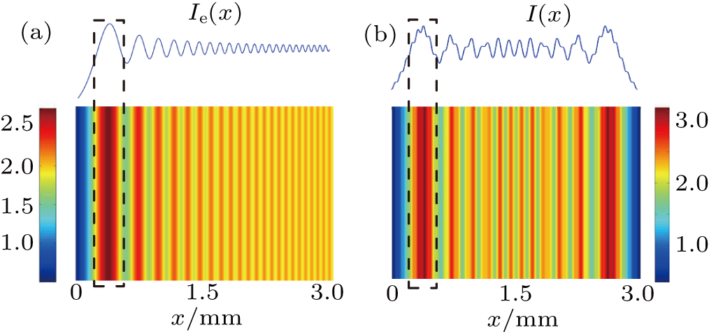
From Eqs. (2) and (4), we obtain the intensity patterns for the Fresnel diffraction by a single edge and a slit and the intensity distribution curves of and , which are shown in Figs. 2(a) and 2(b). On comparing the parts of the two curves within the black dotted markings, we find that their main tendencies are similar; the difference between them is that within the black dotted markings is more complex and contains many small fluctuations, referred to as ripples. The existence of ripples leads to a complex peak position rule.

Fig. 2. (color online) (a) Intensity pattern of Fresnel diffraction by a single edge with λ = 650 nm, and d = 300 mm. (b) Intensity pattern of Fresnel diffraction by a slit with λ = 650 nm, a = 3 mm, and d = 300 mm.

By repeating the above process for various values of d (diffraction distance), a series of intensity patterns are obtained. We produce a series of patterns for a single edge and then obtain the density pattern of Fresnel diffraction by a single edge in the x plane shown in Fig. 3(a). The white dotted line in Fig. 3(a) is the track of the peak points. In a similar manner, we obtain the density pattern of Fresnel diffraction by a slit in the τχ plane, which is shown in Fig. 3(b). The two white solid broken lines denote the accurate tracks of the peak points of the Fresnel diffraction by a slit, and they fluctuate around a white dotted line called as the central line; the amplitude of the fluctuation increases with increase in τ.

Fig. 3. (color online) (a) Density pattern of the Fresnel diffraction by a single edge in the x plane. (b) Density pattern of the Fresnel diffraction by a slit in the τχ plane.

The single edge can be seen as a special slit where . As for the Fresnel diffraction by a slit with fixed values of λ and d, the model of the slit approaches a single edge as a increases, and the white broken line in Fig. 3(b) approaches the white dotted line in Fig. 3(a) as the fluctuating amplitude decreases. However, if the fluctuating amplitude decreases, the white broken line in Fig. 3(b) must approach the central line in Fig. 3(b). Thus, we deduce that the white dotted line in Fig. 3(a) should have the same expression as that of the central line in Fig. 3(b).

In Fig. 3(b), with an increase in τ, the diffraction pattern approaches the Fraunhofer diffraction, and the similarity between the slit aperture and the diffraction pattern decreases. Thus, τ should not be very large. In this study, τ is maintained at a value below 0.2.

2.2. Peak position of Fresnel diffraction by a single edge

According to Ref. [12], the white dotted line shown in Fig. 3(a) is a parabola, and the peak points correspond to . However, the precisely calculated value of Eq. (4) obtained using discretization indicates that the accurate value of α1 is 1.2172. In Section 2.1, we know that the central line in Fig. 3(b) has the same expression as that of the white dotted line shown in Fig. 3(a). Therefore, the central line also fulfils the condition

3. Peak position of Fresnel diffraction by a slit

The expression for m (distance between the peak point and the edge) can be obtained using two methods. In the first method, we deduce the accurate locations of the peak points using the formula for deviation and then obtain the required expression. In the second method, we obtain the expression using the characteristics of the track of the peak points represented by the white solid broken line in Fig. 3(b).

3.1. Expression from the first method

From Eqs. (1) and (3), we obtain the expression for I(χ, τ) at α1 and α2

In the intensity curve shown in Fig. 2(b), the peak point is one of the extreme points of ; therefore, . From the expression , we obtain . Therefore,

and are the same intensity, but are expressed in different forms. Thus, the peak point meets the condition .

On taking the first derivative of Eq. (6) with respect to α1, we obtain

Let Eq. (7)= 0. Thus,
i.e.,
where , and the set of α1n for various values of n are the values of α1 that correspond to the extreme points.

According to Eq. (5), the central line corresponds to α1= 1.2172. Thus, we conjecture that the α1n nearest to 1.2172 corresponds to the peak point, which is denoted as αM

where . We denote the coordinate of the peak point as xM, and . Thus,
where m1 is the distance between the peak point and edge deduced using the first method, and round( ) indicates rounding.

3.2. Expression from the second method

Furthermore, we detect the peak position based on the characteristics of the track of the peak points of the slit represented by the white solid broken line shown in Fig. 3(b).

The existence of fluctuations in Fig. 3(b) depends on the existence of ripples. T is the cycle of the ripple containing the peak point shown in Fig. 4(a).

Fig. 4. (color online) Cycle of ripple and curve mτ.

As shown in Fig. 4(b), with a decrease in τ, the peak point moves gradually from the extreme left to the extreme right at approximately α1= 1.2172, then abruptly jumps to the extreme left, and repeats this process again. The fluctuation at approximately α1= 1.2172 makes the mτ curve fluctuate around the line (corresponding to α1= 1.2172), which is shown in Fig. 4(c). Figure 4(c) is a section of the lines shown in Fig. 3(b). In Fig. 4(c), the value of τ at which the peak point instantaneously jumps is denoted as τ0, the changing amplitude is F, and the distribution is linear between two random adjacent instances of τ0. Thus, if τ0 and F are known, the equation for the broken line in Fig. 4(c) can be clearly expressed.

Moreover, figure 4(b1) shows that m changes from 0.5T on the right to 0.5T on the left, i.e., F = 0.5T+0.5T = T.

We use Eq. (11), which was deduced from the aforementioned first method, to obtain F and τ0. Evidently, the value of changes suddenly when , with the change in the value of , which must correspond to τ0. Therefore,

i.e.,
where

Furthermore, from Eq. (11), we obtain , when ; hence,

Based on Eqs. (13) and (14) and the assumption of linear distribution between two random adjacent instances of τ0, the expression m is deduced as

where m2 is the distance between the peak point and edge deduced using the second method, and frac( ) indicates resolving the fractional part.

4. Simulation
4.1. Analysis of errors

To numerically prove the viability of Eqs. (11) and (15), we provide their error curves as shown in Fig. 5.

Fig. 5. (color online) Error of Eqs. (11) and (15). (a) Difference between Eqs. (11) and (15). (b) Error of Eq. (11).

Figure 5(a) shows that the two expressions in Eqs. (11) and (15) are very similar with a 4-nm difference at . Thus, it is only necessary to show the error of Eq. (11) (the true values are obtained from the peak position of the large sampling discretization model using Kirchhoff’s diffraction theory), which is shown in Fig. 5(b). There are 5641 sampling points in Fig. 5(b), and 60 points have an error greater than with a probability of 60/5641 = 1.06%, i.e., more than 98.94% of the time, the errors in Eqs. (11) and (15) are below .

4.2. Influence of quantization owing to the size of CMOS

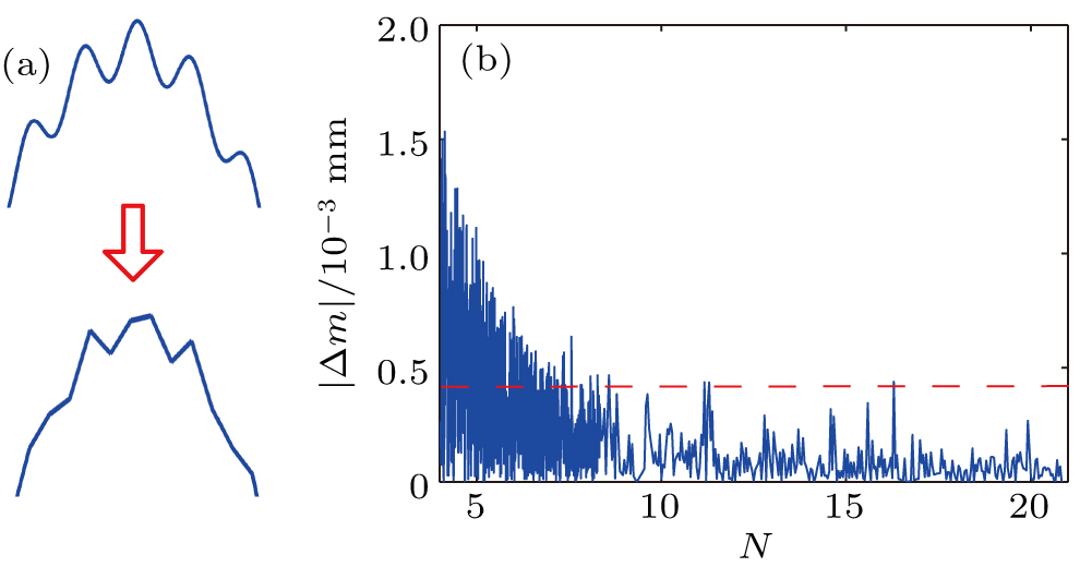
Figure 6(a) shows that the pixel size of the CMOS does not allow the intensity distribution to be smooth because of the decrease in the sample size of the ripple containing the peak point. This phenomenon increases the location error of the peak points.

Fig. 6. (color online) Influence of quantization owing to size of CMOS.

We denote the pixel size of the CMOS as s. Thus, the sampling size of the main peak is

Figure 6(b) represents the curve , where is the error in the value of m (distance between edge and corresponding peak point) caused by the pixel size of the CMOS. It is observed that decreases with the increase in N, and decreases slowly and becomes less than when . This means that N should be greater than a certain value when is limited within a certain range.

4.3. Application conditions of d and a

We can deduce the ranges of d and a that are suitable for our method using some application conditions. The conditions include the requirements for the value of , the limitation of τ shown in Section 2.1, etc.

Condition 1. In Section 4.2, N should be greater than a certain value when is limited within a certain range. From the expression of N shown in Eq. (16), , where N0 is the minimum value of N, and the range of N can be decided based on the requirement of . For example, according to Fig. 6(b), if is required to be less than , N should be greater than 7; thus, .

Condition 2. In section 2.1, the condition has been defined.

Condition 3. In this paper, the diffraction pattern is obtained directly using the CMOS without a lens; therefore, the width of the slit to be measured should be less than the sensor of the CMOS and less than 10 mm, i.e., mm.

Condition 4. The photosensitive surface of the CMOS is at some distance from the end surface; therefore, we set the diffraction distance to be greater than 30 mm, i.e., mm.

In summary, we can obtain suitable ranges for d and a for our method using , 30 mm), and , , 10 mm)]. For example, if nm, the quantization error , and the pixel size of the CMOS , then the slit width that can be measured using this method is in the range from 0.3122 mm to 10 mm.

5. Experiments
5.1. Experimental setup and figures

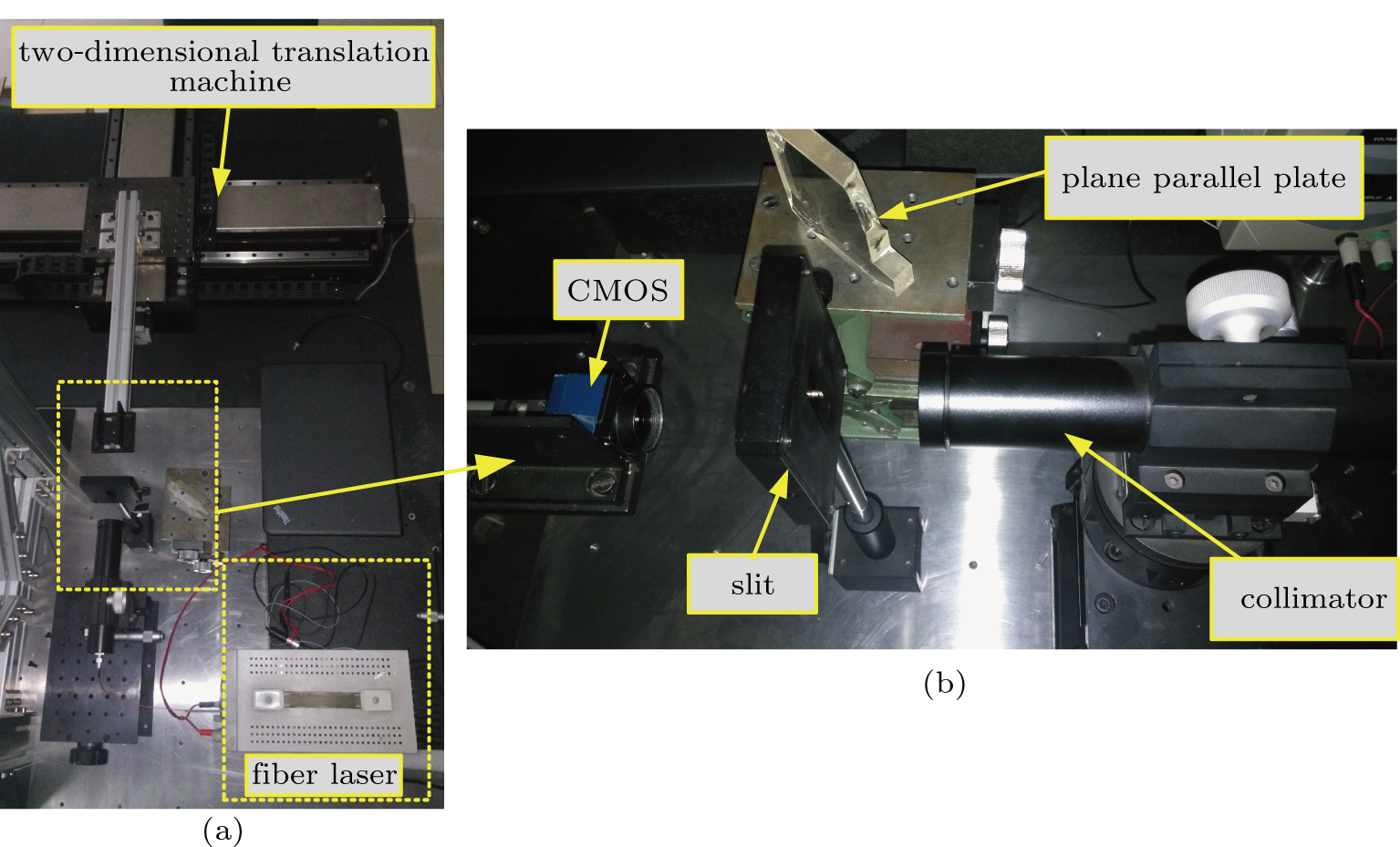
Figure 7(a) shows the experimental setup used in this study, and it corresponds to the sketch of the principle shown in Fig. 1. Figure 7(b) is the enlarged image of the highlighted part of Fig. 7(a).

Fig. 7. (color online) Experimental setup.

In Fig. 7, the light source is a fibre laser with a wavelength of 650 nm. The pixel size of the CMOS is , and the size of the CMOS is 5.3250 mm × 6.6560 mm. The CMOS is set up on a two-dimensional translation machine with a mobile precision of . The nominal size of the slit to be measured is . It should be noted that a plane parallel plate is used to focus the collimator at the beginning of the experiment.

5.2. Experiment figures

A plane parallel plate is one of the simplest lateral shearing interferometers used to obtain qualitative work in a laboratory, and we use it to focus the collimator. The shearing interferogram is shown in Fig. 8(a), and the area of the wavefront overlap appears uniform, which means that focusing has been achieved.

Fig. 8. (color online) Shearing interferogram and diffraction patterns. (a) Shearing interferogram. (b) Diffraction patterns of a slit of width a = 3 mm, and a diffraction distance d ranging from 100 mm to 350 mm with an interval of 50 mm.

We change the diffraction distance d from 100 mm to 500 mm by moving the two-dimensional translation machine with an interval of 5 mm. In order to enhance the SNR, 30 figures are acquired continuously for every value of d, and the mean figure is obtained using the following calculation. Finally, we obtain 81 mean figures, six of which are shown in Fig. 8(b).

5.3. Experiment data

The corresponding values of d and N for λ = 650 nm, a = 3 mm, and (pixel size of CMOS) are shown in Table 1.

Table 1.

Values of τ and sampling size N for various d (mm).

.
5.3.1. Experiment error with 81 mean figures

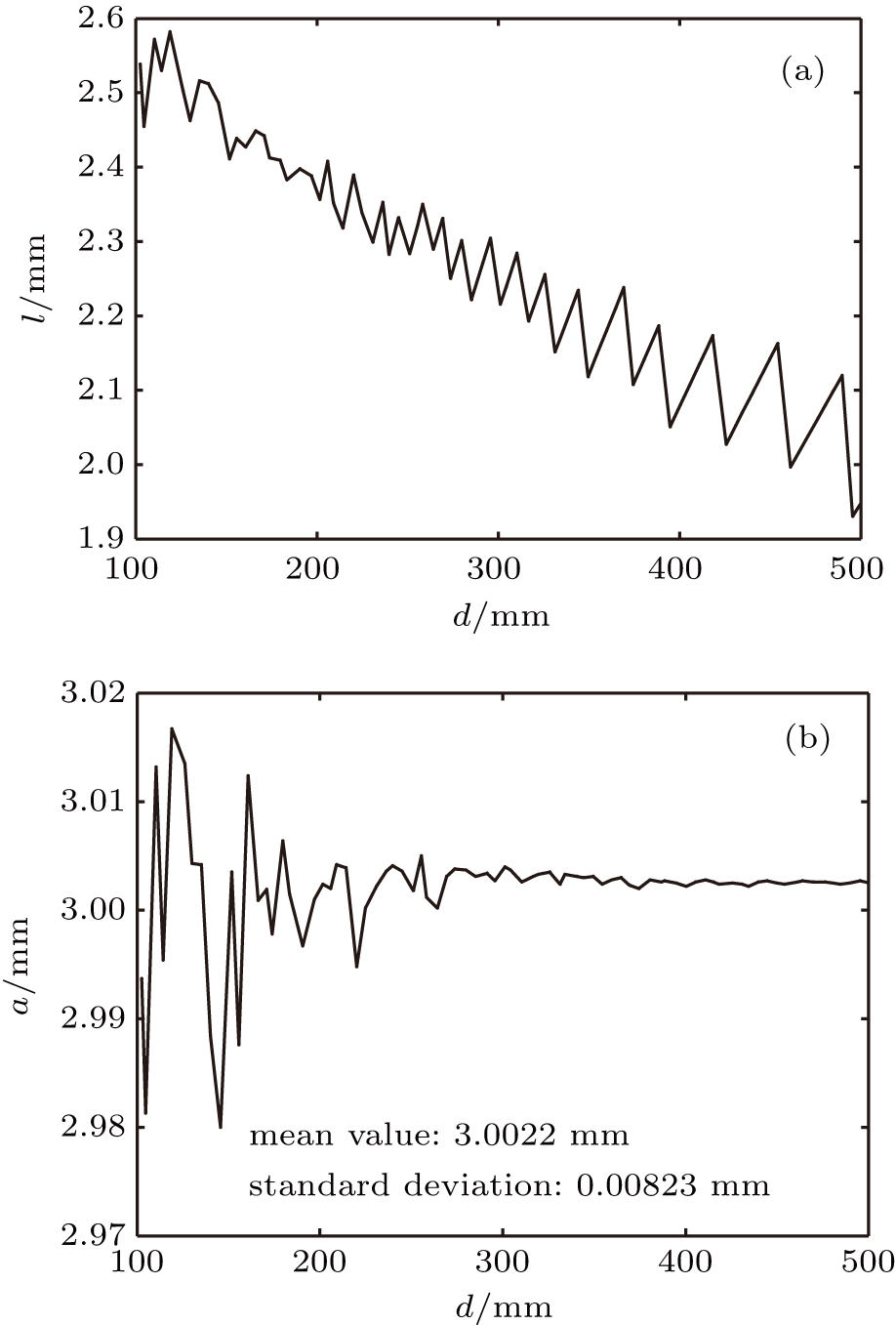
In the beginning, we use all the 81 mean figures for the calculation, and obtain 81 values of l to plot the curves dl (d is the diffraction distance, l is the distance between the two peak points), as shown in Fig. 9(a).

Fig. 9. Experimental curves.

From Eq. (11), we obtain

With the experimental value of l shown in Fig. 9(a), the value of a can be calculated using Eq. (17). The curve da is shown in Fig. 9(b), and the mean value and standard deviation of the 81 values of a are also shown.

From Fig. 9(b), the following can be observed: (i) the measurement result is ( ), which represents the repeatability error of the 81st measurement for various values of d. (ii) The volatility of the measured value of a reduces as d increases (which is proportional to N), i.e., the error decreases as N increases.

Furthermore, in order to verify the accuracy of Eqs. (11) and (15) using the experiment, we process the data as follows: we denote the mean value of a in Fig. 9(b) as (which is the true value of the slit width) and calculate the experimental values of (m is the distance between peak point and edge, and l is the distance of the two peak points shown in Fig. 9(a)), which is shown in Fig. 10(a).

Fig. 10. (color online) (a) Experimental curve and (b) error curve.

In Fig. 10(a), the function curve is calculated using the value of and Eq. (11). The difference between the two curves in Fig. 10(a) is shown in Fig. 10(b). From Fig. 10(b), we can see that the experimental error of m decreases with an increase in d (which is proportional to N), and the error is below when (corresponding to ).

5.3.2. Experiment error with 11 mean figures

From Fig. 9(b), the error decreases with the increase in d. Therefore, we sample the 81 mean figures within different small regions of d and calculate the mean value of a and the corresponding deviation. The regions and corresponding results are shown in Table 2.

Table 2.

Mean values and standard deviations.

.

From Table 2, 8 regions are obtained and 11 values of a are used in any region. The standard deviation represents the repetition error of the measurement, and the data shows that the repetition errors decrease with an increase in d (which is proportional to N) and reaches at mm. Thus, the measured value of the slit is .

Overall, the experimental values of m are in good agreement with Eqs. (11) and (15), and the error is below when (where N is the sample size of the ripple containing the peak point). Furthermore, the expression for m shown in Eqs. (11) and (15) can be used to measure the slit width, and the experiment data shows that the repetition accuracy can reach a sub-micro level (the repeatability error for this experiment reached ).

6. Conclusions and outlook

In summary, we numerically deduce the intensity distribution of the Fresnel diffraction by a slit and propose two types of expressions for the edge and peak points. The simulations suggest that the error of the expression is approximately less than at , and the pixel size of the CMOS causes a quantization error in m, which decreases with the increase in the sample size of the ripple containing the peak point.

We also use an expression to detect the contour of the slit. A slit with a nominal width of 3 mm is used, and the experimental data reveal that the repeatability error of the measurement decreases as d increases, and it reaches when mm.

In future research, instead of a slit, we intend to use an aspheric surface as the diffraction object and suggest a new method for testing the aspheric surface by detecting the peak point of the corresponding Fresnel diffraction pattern.

Reference
[1] Liu J 2016 Chin. Phys. 25 076106
[2] Diemoz P C Vittoria F A Olivo A 2014 Opt. Express 22 15514
[3] Gayer C W Hemmers D Stelzmann C Pretzler G 2013 Opt. Lett. 38 1563
[4] Lee W K Cloethens P Schlenker M 2004 Acta Cryst. 60 58
[5] Langlois P Lessard R A Boivin A 1985 Appl. Opt. 24 1107
[6] Fukaya J Sasaki A Matsuda Y Aoyama H 1985 Appl. Opt. 34 7820
[7] Xie Y Zakharian A R Moloney J V Mansuripur M 2004 Opt. Express 12 6106
[8] Chen J Kuang D F Fang Z L 2009 Chin. Phys. Lett. 26 094210
[9] Pu J X Cai C Hu X D Liu X Y 2005 Chin. Phys. Lett. 22 2259
[10] Teng S Y Cheng C F Liu M Liu L R Xu Z Z 2003 Acta Phys. Sin. 52 316 in Chinese
[11] Song H S Liu M Liu G Y Xu Z W Teng S Y Cheng C F 2010 Chin. Phys. 19 124202
[12] Case W B Sadurni E Schleich W P 2012 Opt. Express 20 27253
[13] Modregger P Lubbert D Schafer P Kohler R Weitkamp T Hanke M Baumbach T 2008 Opt. Express 16 5141
[14] Shimobaba T Masuda N Ito T 2012 Opt. Express 20 9335
[15] Umul Y Z 2005 Opt. Express 13 8469
[16] Maqsood M W Mehfuz R Chau K J 2010 Opt. Express 18 21669
[17] Wang Z L Zhou M Gao C Y Zhang W 2012 Chin. Phys. 21 064202
[18] Lei Z M Sun X Y Lv F N Zhang Z Lu X Q 2016 Chin. Phys. 25 114201
[19] Song Y Hao Q Li D C 2006 Proc. 6150
[20] Southwell W H 1981 J. Opt. Soc. Am. 71 7
[21] Xie J H Zhao D Z Yan J X 2012 Physical Optics Coursebook Beijing Beijing Institute of Technology Press 220 222 in Chinese